Week 5 - Rayleigh Taylor Instability
AIM:
- To list the practical CFD models that have been based on the mathematical analysis of Rayleigh Taylor waves and mathematical models have been adapted for CFD calculations.
- To perform the Rayleigh Taylor instability simulation for 2 different mesh sizes with the base mesh being 0.5 mm. Compare the results by showing the animations.
- Observe the differences in the animation and explain the effect of mesh size on simulation.
- Also, explain why a steady-state approach might not be suitable for these types of simulation.
- Run one more simulation with water and user-defined material(density = 400 kg/m3, viscosity = 0.001 kg/m-s) for refined mesh.
- Define the Atwood Number. Find out the Atwood number for both the cases and explain how the variation in Atwood number in the above two cases affects the behavior of the instability
------------------------------------------------------------------------------------------------------------------------------------------------------
The Rayleigh–Taylor instability, or RT instability, is an instability of an interface between two fluids of different densities which occurs when the lighter fluid is pushing the heavier fluid. Examples include the behavior of water suspended above oil in the gravity of Earth, mushroom clouds like those from volcanic eruptions and atmospheric nuclear explosions, supernova explosions in which expanding core gas is accelerated into denser shell gas, instabilities in plasma fusion reactors and inertial confinement fusion.
Water suspended atop oil is an everyday example of Rayleigh–Taylor instability, and it may be modeled by two completely plane-parallel layers of immiscible fluid, the more dense on top of the less dense one and both subject to the Earth's gravity. The equilibrium here is unstable to any perturbations or disturbances of the interface: if a parcel of heavier fluid is displaced downward with an equal volume of lighter fluid displaced upwards, the potential energy of the configuration is lower than the initial state. Thus the disturbance will grow and lead to a further release of potential energy, as the more dense material moves down under the (effective) gravitational field, and the less dense material is further displaced upwards. This was the set-up as studied by Lord Rayleigh. The important insight by G. I. Taylor was his realisation that this situation is equivalent to the situation when the fluids are accelerated, with the less dense fluid accelerating into the more dense fluid. This occurs deep underwater on the surface of an expanding bubble and in a nuclear explosion.
As the RT instability develops, the initial perturbations progress from a linear growth phase into a non-linear growth phase, eventually developing "plumes" flowing upwards (in the gravitational buoyancy sense) and "spikes" falling downwards. In the linear phase, the fluid movement can be closely approximated by linear equations, and the amplitude of perturbations is growing exponentially with time. In the non-linear phase, perturbation amplitude is too large for a linear approximation, and non-linear equations are required to describe fluid motions. In general, the density disparity between the fluids determines the structure of the subsequent non-linear RT instability flows (assuming other variables such as surface tension and viscosity are negligible here). The difference in the fluid densities divided by their sum is defined as the Atwood number, A. For A close to 0, RT instability flows take the form of symmetric "fingers" of fluid; for A close to 1, the much lighter fluid "below" the heavier fluid takes the form of larger bubble-like plumes.
Models that have been adapted from the R-T waves model are,
- Richmyer-Meshkov instability
- Plateau-Rayleigh instability
- Kelvin-Helmhontz instability
Richmyer-Meshkov instability
The Richtmyer-Meshkov instability arises when a shock wave interacts with an interface separating two different fluids. It combines compressible phenomena, such as shock interaction and refraction, with hydrodynamic instability, including nonlinear growth and subsequent transition to turbulence, across a wide range of Mach numbers. This review focuses on the basic physical processes underlying the onset and development of the Richtmyer-Meshkov instability in simple geometries. It examines the principal theoretical results along with their experimental and numerical validation. It also discusses the different experimental approaches and techniques and how they can be used to resolve outstanding issues in this field.
Plateau-Rayleigh instability
A liquid jet, initially of constant radius, is falling vertically under gravity. The liquid length increases and reaches a critical value. At this critical value, the jet loses its cylindrical shape as it decomposes into a stream of droplets. This phenomenon occurs primarily as a result of surface tension. Joseph Plateau first characterized this instability in 1873 through experimental observation, building on the work of Savart. He noted the instability arose when the liquid column length exceeded the column diameter by a factor of about 3.13 (Plateau, 1873). Lord Rayleigh later corroborated Plateau’s work, giving an analytical explanation of this physical observation. This liquid behavior derives from the existence of small perturbations in any physical system. All real-world flows have some non-negligible external disturbance that will increase
exponentially in unstable systems. In general, this deformation of the column, called varicose perturbations, is represented as a series of periodic displacement sinusoids. For certain wavelengths, these perturbation waves will grow larger in time.
Kelvin-Helmhontz instability
The Kelvin–Helmholtz instability typically occurs when there is velocity shear in a single continuous fluid, or additionally where there is a velocity difference across the interface between two fluids. A common example is seen when wind blows across a water surface; the instability constant manifests as waves. Kelvin-Helmholtz instabilities are also visible in the atmospheres of planets and moons, such as in cloud formations on Earth or the Red Spot on Jupiter, and the atmospheres (coronas) of stars, including the sun's.
Basic Setup:
The geometry is initially drawn in Space Claim using the following guidlines given in the video.
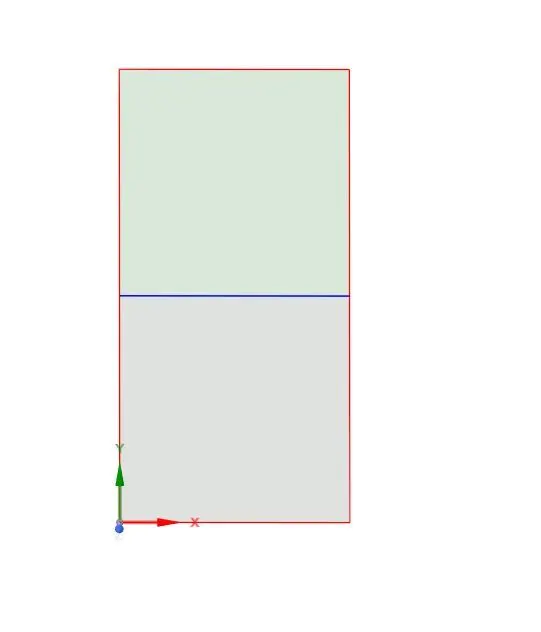
The dimensions are 40mm X 20mm. The line in the center acts as the separation layer between the 2 phases.
We use share topology to ensure data exchange takes lace between the 2 phases.
MESH:
- The basic mesh size is set to 0.5mm to just check and study th development of the RT wave.
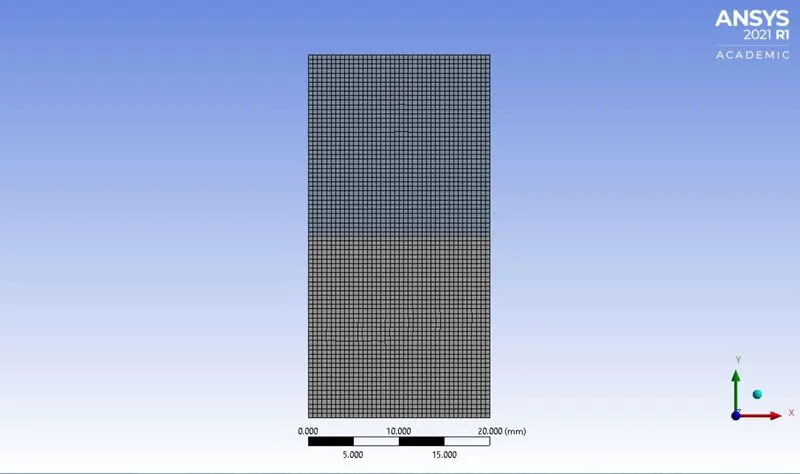
- The refiend mesh was set to 0.2 mm to study the effect of the RT waves.
Basic Setup on Fluent:
- Once the previous steps have been implemented,the fluent module is opened.
- Most of the required information such as values of density, velocity etc. are inputed in this module.
- The laminar model was selected.
- Initially we setup the reference values as dipicted below:
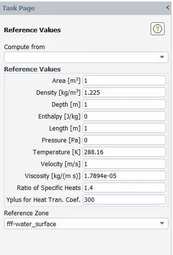
- Once we set the reference values, we also make sure to seup the matrial required and the boundary conditions.
- Post this step we run the simulation for 300 step with a time step size of 0.005sec utilizing the SIMPLE method. This is done as this method is not computationally expensive and dosen't consume much time.
- This setup is done in transient setting.
CASE 1:
Mesh size 0.5
Material: Water and Air
Statistics:

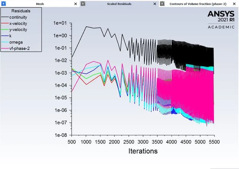
Residuals:
Start Phase:
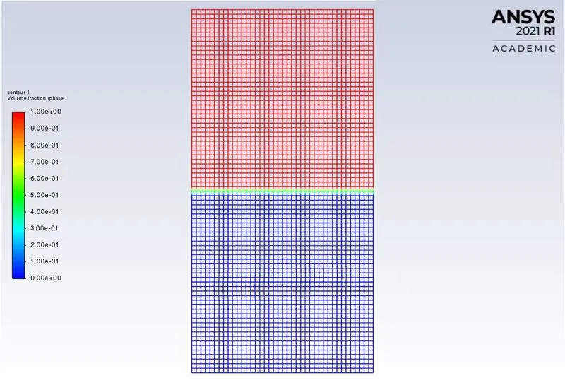
End Phase:
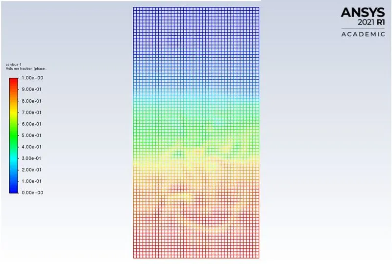
Simulation:
CASE 2:
Mesh size: 0.2mm
Material: Water and Air
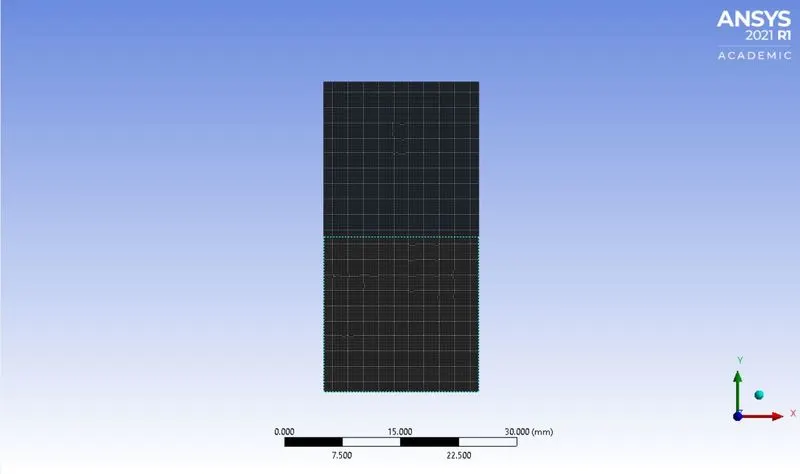
Statistics:

Residuals:
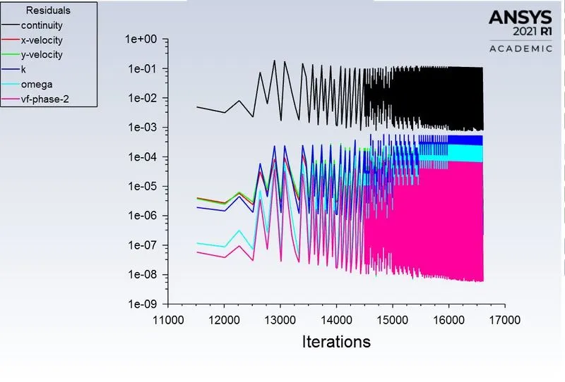
Start Phase:
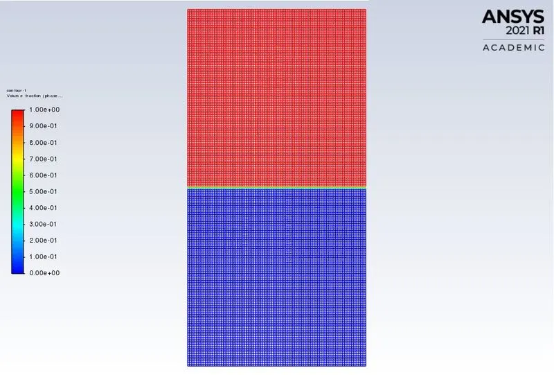
End Phase:
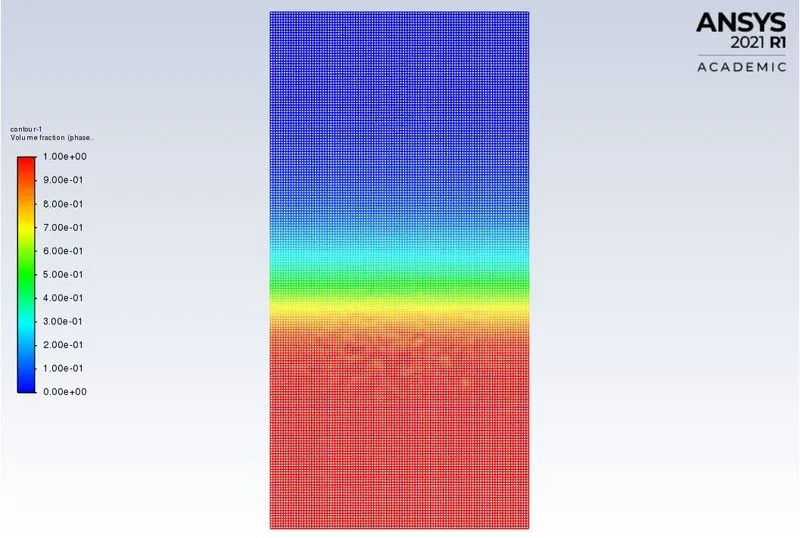
Simulation:
CASE 2:
Mesh size: 0.2 mm
Material: Water and user defiend material
Statistics:
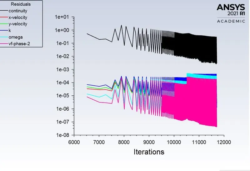
Residuals:
Start Phase:
End Phase:
Simulation:
OBSERVATIONS:
- The basic understanding of this project is the formation of instability when a lighter fluid displaces a heavier fluid and how the patterns of waves are formed.
- This we study in varying mesh sizes.
- The most important aspect to observe is the instability in various mesh sizes.
- It was observed that the instability was much more pronounced when the mesh size was finer.
- The most important aspect is toensure that the fluid has mixed properly. This is better observed when the mesh is fine.
- So from this we can conclude that the finer the mesh size, the smoother is the animation and accurate is the result.
Steady State Analysis:
- Steady state analysis is generally used to study the initial and final results of a problem.
- In this case we are interested to study the evolution of the wave at every time step.
- This is possible only with a transient simulation.
- Also we cannot control the timestep as in transient simulations.
Hence the above are the reasons for not being able to use a steady simulation.
Atwood Number:
The Atwood number (A) is a dimensionless number in fluid dynamics used in the study of hydrodynamic instabilities in density stratified flows. It is a dimensionless density ratio defined as
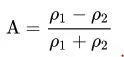
where
- ρ 1 {\displaystyle \rho _{1}}
 = density of heavier fluid
 - ρ 2 {\displaystyle \rho _{2}}
 = density of lighter fluid
CASE 1:
Materials:
- Air
- Water
= 998.2`Kg/m^3` [Water]
ρ 2 {\displaystyle \rho _{2}} = 1.225`Kg/m^3` [Air]
A=[998.2-1.225]/[998.2+1.225]
A=0.997
CASE 2:
Materials:
- Water
- User defiend material
= 998.2`Kg/m^3` [Water]
ρ 2 {\displaystyle \rho _{2}} = 400`Kg/m^3` [Air]
A=[998.2-400]/[998.2+400]
A=0.427
Variation in Atwood number in the above two cases affects the behavior of the instability.
As the RT instability develops, the initial perturbations progress from a linear growth phase into a non-linear growth phase, eventually developing "plumes" flowing upwards (in the gravitational buoyancy sense) and "spikes" falling downwards. In the linear phase, the fluid movement can be closely approximated by linear equations, and the amplitude of perturbations is growing exponentially with time. In the non-linear phase, perturbation amplitude is too large for a linear approximation, and non-linear equations are required to describe fluid motions. In general, the density disparity between the fluids determines the structure of the subsequent non-linear RT instability flows (assuming other variables such as surface tension and viscosity are negligible here). The difference in the fluid densities divided by their sum is defined as the Atwood number, A. For A close to 0, RT instability flows take the form of symmetric "fingers" of fluid; for A close to 1, the much lighter fluid "below" the heavier fluid takes the form of larger bubble-like plumes.[2]
For lower Atwood number (water-user defiend material mixture) the shapes of the plumes and spikes remain similar and the disturbances are linear for a significant ampunt of time. In the case of higher atwood number the bubble is formed by the ligher material and is formed at a faster pace which increases non linearity in wave propogation.