Week 5 - Rayleigh Taylor Instability

Aim:

To investigate the notion of Rayleigh Taylor instability and some practical CFD models based on Rayleigh Taylor wave mathematical analysis.
To compare the outcomes of the Rayleigh Taylor instability simulation for two different mesh sizes in addition to the baseline.
To investigate the impact of Atwood number variation on Rayleigh Taylor instability in all scenarios.

Aout task:

Rayleigh Taylor instability arises at the interface of two fluids of differing densities when the lighter fluid pushes the heavier fluid. Newton's law of viscosity states that a fluid cannot withstand even the tiniest shear stress, and density is one of the fluid's primary qualities for incorporating shear force. When lighter and heavier fluids are mixed together, the denser fluid rises to the top of the lighter fluid due to gravity, and the density variation at the liquid's interface is unstable. Rayleigh Taylor instability refers to the instability of the interface between various densities of fluid as the lighter fluid is propelled towards the heavier fluid.

Procedure

To get the desirable results we go through 3 major steps in the same sequel and based on the steps we followed during whole setup we got the results.

1. First of all, open the workbench
2. Drag the Fluid Flow (fluent) part in the Project schematic window
3. So, via going through Geometry option open the Space claim
4. Go to the open – new – go to geometry location – select open command
5. By following step 4 we will able to open the geometry in the space claim
6. Now choose the required volume from the whole geometry to do further process efficiently.
7. Check for any overlaps and the intersections that cause problem in the meshing.
8. After verifying the model and then close the window.
9. Now open Ansys Meshing and let the geometry upload.
10. Then firstly name all the parts of the model.
11. Then from the Tree right click on mesh and tap "Generate mesh"
12. Set the sizing of the meshing from its detail and then repeat the step 11.
13. After verifying the mesh, close the Ansys Meshing window.
14. Now open Ansys fluent window by clicking over ‘Setup’ and let the geometry upload.
15. For verifying the check click of ‘Checks’ option and see the results in console.
16. Go to the General and set the case accordingly as mentioned in the challenge
17. As we are dealing with temperature so mark the Energy option and chose the viscous flow option to define the fluid flow.
18. After this set the Boundary conditions.
19. Generated the graphs that we want to observe during the case run.
20. With this go to the results and create a plan in from the centre of the body and allow to show the velocity contour pattern over it during the case run time.
21. In addition to this, from ‘solving’ section also select animation for the same velocity contour.
22. The initialize the case
23. Set the total no. of iteration.
24. Click calculate to make simulation run
25. As the simulation completed close the tab and do the postprocessing as analyse the contours and plots.
26. For this select the plane slice that is situated in the centre of the geometry and over it we have to perform the contour analysis.
27. Close the tab after extracting useful results.
28. Save the case and cut the software.

Results:

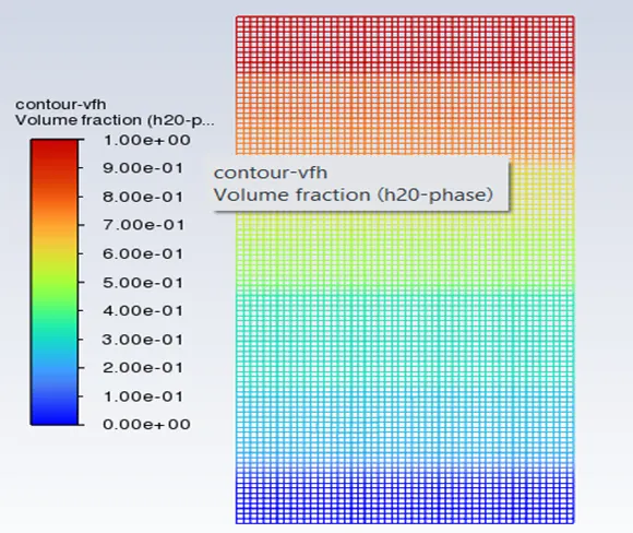
Rest complete case results are attached in word file

Thanks

Anubhav