Week 5 - Rayleigh Taylor Instability

Aim of the challenge:

To Perform the Rayleigh Taylor instability simulation for 2 different mesh sizes with the base mesh of 0.5 mm.

Objectives :

1. The first objective is to simulate a two-dimensional Rayleigh-Taylor instability problem using the classical method of Finite Element analysis of a multiphase model using ANSYS FLUENT.

2. To develop a numerical case set-up for Rayleigh-Taylor instability problem in Ansys Fluent.

3. To conduct grid dependency test to understand the variation in RT instabilites.

4. To understand the effect on RT instabilities due to variation in Atwood number.

Introduction of the challenge

What exactly is Rayleigh-Taylor Instability :

• In Multiphase flow, the dynamic variables like the velocity, viscosity, pressure and density are generally used to explain the movement of fluids under the gravitational field.
• Multiphase flows takes place in nuclear geothermal power plants, food processing industries and many others. One of the basic example is Rayleigh Taylor Instability.

Fig (a): Rayleigh-Taylor Instability

In fig (a), fluid with blue color represents lighter fluid

The fluid in red color represents heavier fluid

• The Rayleigh Taylor Instability is a hydrodynamic instability arises when a high density fluid is placed over a low density fluid in a gravitational field and the two fluids must be immiscible.
• Intially at time t= 0, the system of two fluids is in hydrostatic equlibrium. The pressure gradients are balanced and fluid is in static equilibrium.
• When the density interface is disturbed, the hydrostatic pressure is generated, so the heavier fluid moves downwards and mixes with the lighter one, with the amplitude of perturbation initially growing exponentially but after sometime saturates and forms characteristic mushroom shape.
• When a heavier fluid is displaced downward with an equal volume of lighter fluid displaced upwards, it results in decrease of potential energy than it’s initial state.
• This RTI has been applied to a wide range of problems including the mushroom clouds like volcanic eruptions, nuclear explosions and plasma fusion reactors instability.

Atwood Number :

Dealing with mixtures of fluid one uses the Atwood number to characterize the density difference between two fluids.

Assume that ρ2">ρ2 is the density of the heavier fluid.
The definition is: At = ρ2-ρ1ρ2+ρ1">ρ2−ρ1ρ2+ρ12-12+1.

• For more density differences At tends to 1.
• For small differences At tends to zero.

Literature Studies made for this :

• The RTI phenomenon was initially introduced by Rayleigh 1883 and later was observed for all accelerated fluids by Taylor 1950.
• Indrashis Saha 2020 study of Rayleigh Taylor Instability with the help of CFD simulation and was well validated with experimental results.

Case studies :

Task1 :

Subtask 1 :

to Effect of mesh refinement over CFD results.

Subtask 2 :

In this study, the results obtained from Subcase 1 and Subcase 2 will be evaluated on the basis of mesh refinement.

task2 : main effect of Atwood number over Rayleigh-Taylor instabilities.

For same mesh characteristics the two case set-up's (Subtask 2 and yask2) with different Atwood number will be evaluated to understand the effect on Rayleigh-Taylor instabilities.

task set-up :

• Solver- Pressure based and absolute velocity is used. Transient state calculation.Gravity is enabled in -ve Y-axis.
• Multiphase model is turned on along with volume of fluid and number of Eulerian phases is chosen as 2. Accordingly, implicit scheme is selected.Viscous model- Laminar is used
• Patching of the volume of the two phases is performed before start of the simulation.
• Air and Water are the two phase used.
• Then patch the surfaces. volume fraction of "1" is taken for water surface and "0" for air surface.

Why we not steady-state calculation?

The steady state calculations are useful when the study is focused on to calculate / simulate the end results. Here in this study, the instabilities information is sensitive and completely time-dependent. At each and every time step, the instabilities grow exponentially. T

[A] Pre-Processing of challenge:

Geometry :

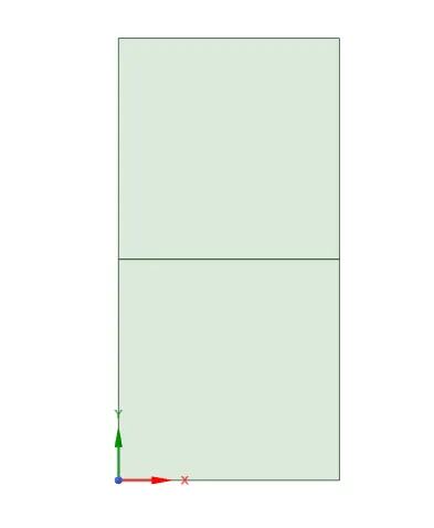
• Geometry is generated in spaceclaim with a dimension of 20x20.Two squares has been created in such a way that it is placed one over the other.After that pull tool is used to convert a sketch into surfaces.
• Then share the topology between two surfaces for the effective transfer of information and to connect a mesh between two interfaces.

Mesh :

Task 1 :

Subtask1 :

1.1.1 Details :

Mesh	Coarse
Element size	0.5 mm
Number of elements	3200
Density of primary fluid	Air (1.225 kg/m3">m3�3)
Density of secondary fluid	Water (998.2 kg/m3">m3�3)
Atwood number	0.9975

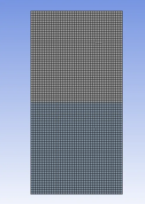
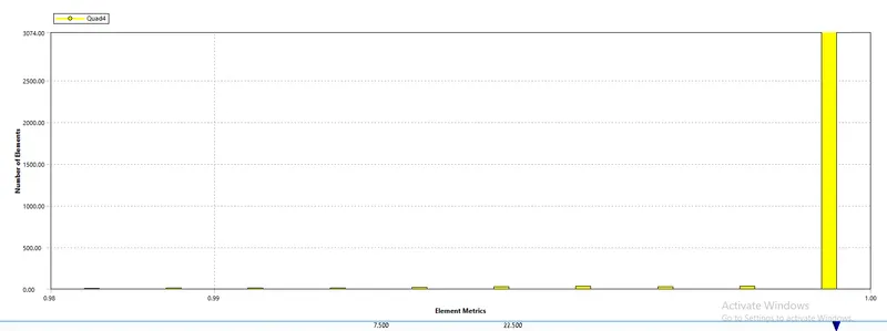
Mesh quality :

STEP 3 : SETUP

SETUP
Solver Type	Pressure-Based
Velocity Formulation	Absolute
Time	Unsteady
Models	Viscous model : laminar Multiphase : Volume of fluid : Implicit formulation : 2 phases
Material	Fluid type : Air : water liquid Solid-type : Aluminium
Cell zones	Fluid type : Air : water
Boundaries	Standard
Reference values	Standard
Initialization	Standard
Patch	Water-surface (1 value of volume fraction of water) Air-surface (0 value of volume fraction of water)

Note : The above table is for case 1 .

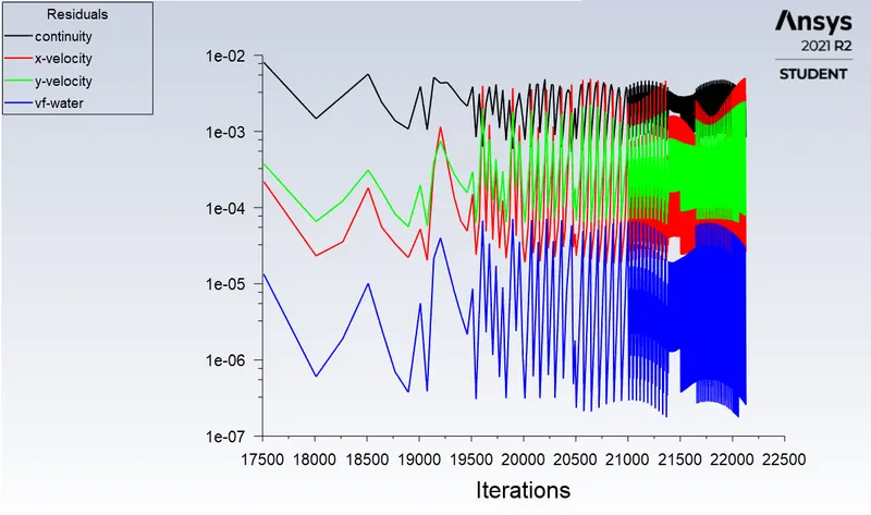
Residual plot :

SubTask 2 :

1.2.1 Details :

Mesh	Refined
Element size	0.18 mm
Number of elements	24642
Density of primary fluid	Air (1.225 kg/m3">m3)
Density of secondary fluid	Water (998.2 kg/m3">m3)
Atwood number	0.9975

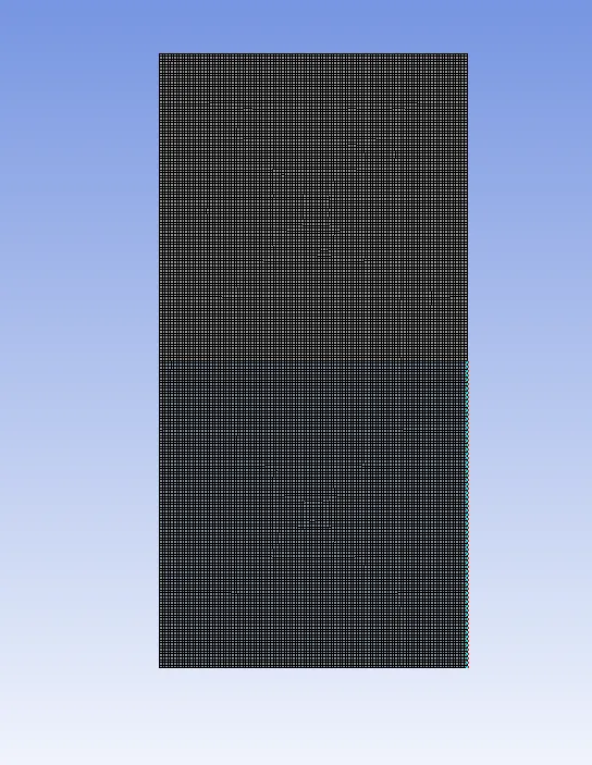
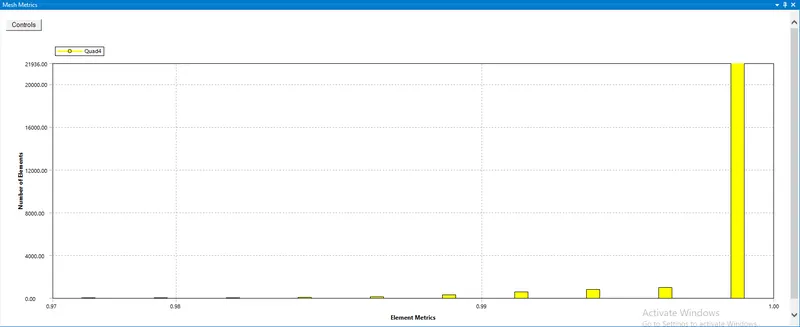
Mesh quality :

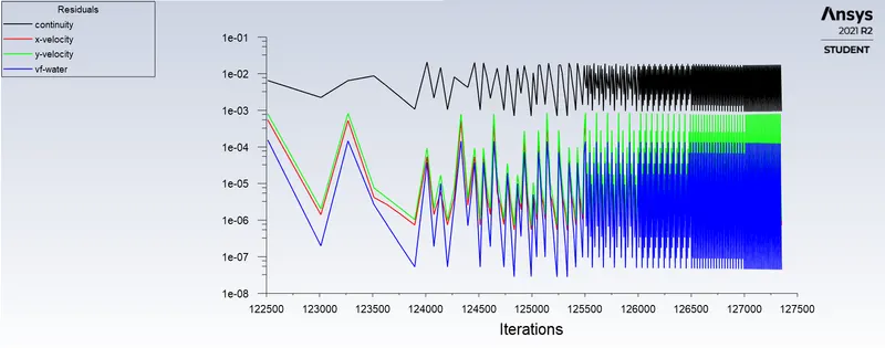
Residuals :

Task2 :

2.1 Details :

Mesh	Refined
Element size	0.18 mm
Number of elements	24642
Density of primary fluid	User-defined (400 kg/m3">m3)
Density of secondary fluid	Water (998.2 kg/m3">m3)
Atwood number	0.4278

STEP 3 :

SETUP
Solver Type	Pressure-Based
Velocity Formulation	Absolute
Time	Un-Steady
Models	Viscous model : laminar Multiphase : Volume of fluid : Implicit formulation : 2 phases
Material	Fluid type : user-defined : water liquid Solid-type : Aluminium
Cell zones	Fluid type : Air : water
Boundaries	Standard
Reference values	Standard
Initialization	Standard
Patch	Water-surface (1 value of volume fraction of water) Air-surface (0 value of volume fraction of water)

Conclusion :

• Steady state solution determines the fully developed solution.This numerical simulation was validated with the observations obtained by previous researchers and this was done by the variation in Atwood Number where we obtained the same observation. In lower Atwood numbers, spikes and globules were still present at the end of the simulation which was not there in Atwood Number of 0.9 in Case 1.

1. -phase flows with large density ratios. Journal of Computational Physics, 226(2), 2078-2095.