Week 5 - Rayleigh Taylor Instability

AIM:

• To mention some practical CFD models that have been based on the mathematical analysis of Rayleigh Taylor waves and explain how these mathematical models have been adapted for CFD calculations.
• To perform the Rayleigh Taylor instability simulation for 2 different mesh sizes with the base mesh being 0.5 mm and compare the results by showing the animations.
• To run one more simulation with water and user-defined material(density = 400 kg/m³, viscosity = 0.001 kg/m-s) for refined mesh.
• To define the Atwood Number and find out the Atwood number for both the cases and explain how the variation in Atwood number in the above two cases affects the behavior of the instability.

SOLUTION:

1. What are some practical CFD models that have been based on the mathematical analysis of Rayleigh Taylor waves? In your own words, explain how these mathematical models have been adapted for CFD calculations.

Rayleigh Taylor instability:

• The Rayleigh–Taylor instability, or RT instability is an instability of an interface between two fluids of different densities which occurs when the lighter fluid is pushing the heavier fluid.
• Examples include the behavior of water suspended above oil in the gravity of Earth, mushroom clouds like those from volcanic eruptions and atmospheric nuclear explosions, supernova explosions in which expanding core gas is accelerated into denser shell gas, instabilities in plasma fusion reactors and inertial confinement fusion.
• Water suspended atop oil is an everyday example of Rayleigh–Taylor instability, and it may be modeled by two completely plane-parallel layers of immiscible fluid, the denser fluid on top of the less dense one and both subject to the Earth's gravity.
• As the RT instability develops, the initial perturbations progress from a linear growth phase into a non-linear growth phase, eventually developing "plumes" flowing upwards (in the gravitational buoyancy sense) and "spikes" falling downwards. In the linear phase, the fluid movement can be closely approximated by linear equations, and the amplitude of perturbations is growing exponentially with time. In the non-linear phase, perturbation amplitude is too large for a linear approximation, and non-linear equations are required to describe fluid motions.

Some practical CFD models that have been based on the mathematical analysis of Rayleigh Taylor waves:

• Saffman–Taylor instability
• Richtmyer–Meshkov instability
• Kelvin–Helmholtz instability
• Mushroom cloud
• Plateau–Rayleigh instability
• Salt fingering
• Hydrodynamic stability
• Kármán vortex street
• Fluid thread breakup

Saffman–Taylor instability:

The Saffman–Taylor instability, also known as viscous fingering, is the formation of patterns in a morphologically unstable interface between two fluids in a porous medium.

It occurs when a less viscous fluid is injected, displacing a more viscous fluid; in the inverse situation, with the more viscous displacing the other, the interface is stable and no instability is seen. Essentially the same effect occurs driven by gravity (without injection) if the interface is horizontal and separates two fluids of different densities, the heavier one being above the other: this is known as the Rayleigh-Taylor instability.

Most experimental research on viscous fingering has been performed on Hele-Shaw cells, which consist of two closely spaced, parallel sheets of glass containing a viscous fluid. The Saffman–Taylor instability is usually seen in an axisymmetric context as opposed to the simple planar case.

Richtmyer–Meshkov instability:

The Richtmyer–Meshkov instability (RMI) occurs when two fluids of different density are impulsively accelerated. Normally this is by the passage of a shock wave. The development of the instability begins with small amplitude perturbations which initially grow linearly with time. This is followed by a nonlinear regime with bubbles appearing in the case of a light fluid penetrating a heavy fluid, and with spikes appearing in the case of a heavy fluid penetrating a light fluid. A chaotic regime eventually is reached and the two fluids mix. This instability can be considered the impulsive-acceleration limit of the Rayleigh–Taylor instability.

Example:

During the implosion of an inertial confinement fusion target, the hot shell material surrounding the cold D-T fuel layer is shock-accelerated. This instability is also seen in Magnetized target fusion.

Kelvin–Helmholtz instability:

The Kelvin–Helmholtz instability is a fluid instability that occurs when there is velocity shear in a single continuous fluid or a velocity difference across the interface between two fluids. Kelvin-Helmholtz instabilities are visible in the atmospheres of planets and moons, such as in cloud formations on Earth or the Red Spot on Jupiter, and the atmospheres of the Sun and other stars

Plateau–Rayleigh instability:

The Plateau–Rayleigh instability, often just called the Rayleigh instability, explains why and how a falling stream of fluid breaks up into smaller packets with the same volume but less surface area. It is related to the Rayleigh–Taylor instability and is part of a greater branch of fluid dynamics concerned with fluid thread breakup. This fluid instability is exploited in the design of a particular type of ink jet technology whereby a jet of liquid is perturbed into a steady stream of droplets.

The driving force of the Plateau–Rayleigh instability is that liquids, by virtue of their surface tensions, tend to minimize their surface area. A considerable amount of work has been done recently on the final pinching profile by attacking it with self-similar solutions.

2. Rayleigh Taylor instability simulation (mesh size = 0.5)

Geometry:

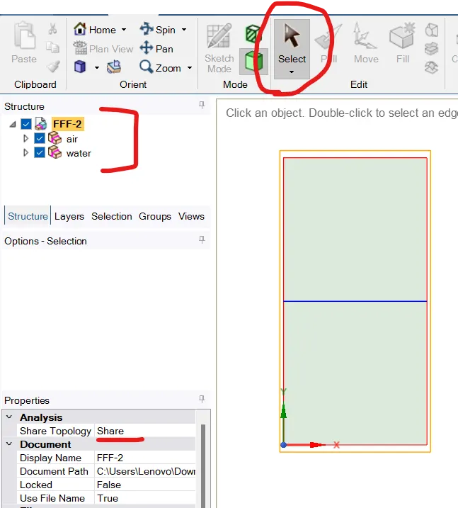
• Draw a square of 20mm and use pull tool to name it as 'air'. Now draw another square of same dimension and use pull tool to name 'water'.
• Now select both the squares and select share for conformal mesh for 'Share topology'. Check whether the surfaces are shared in the 'Share topology' option.
• Make this geometry in 2D in X-Y plane.

Mesh:

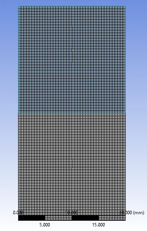
Change the mesh size to 0.5 mm from the default size.

Setup:

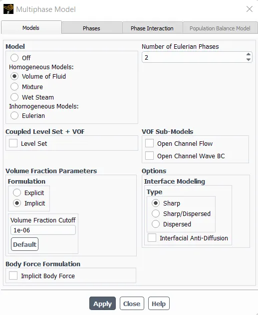
Multiphase:

Homogeneous model: Volume of fluid

Formulation: Implicit

Primary phase: air

Secondary phase: water

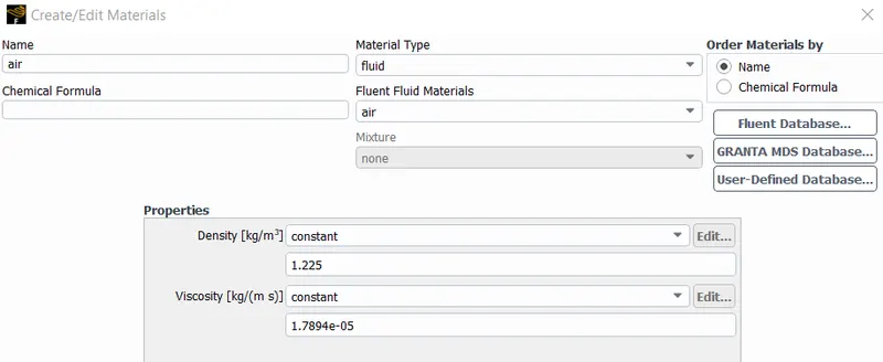
Material Selection:

Primary fluid: Air

Secondary fluid: water

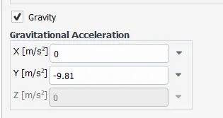
Gravity selection:

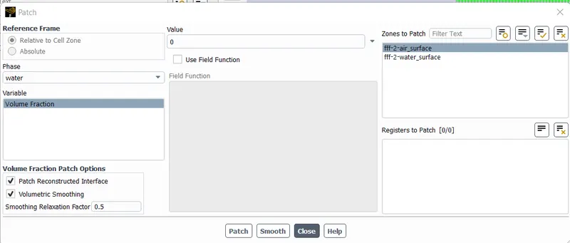
Patch:

After initializing, select patching. Select volume fraction. For air, select 0 and for water select 1 as the fraction.

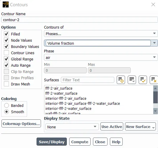
Contours:

After initializing and patching, go to contours and select phases with volume fraction to display the contour plot.

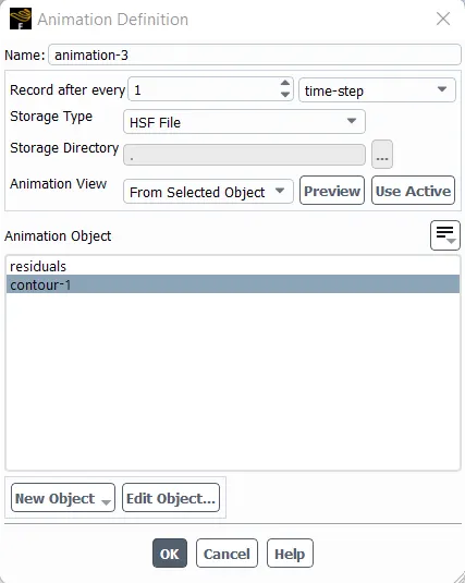
Solution animation:

Create solution animation in the solution icon for contours.

Reacod after every 1 time step.

After making alteration in all the above, hit calculate and proceed with simulation.

Solution:

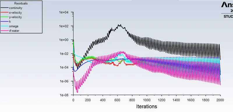
Scaled residuals:

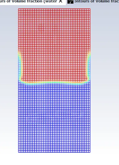
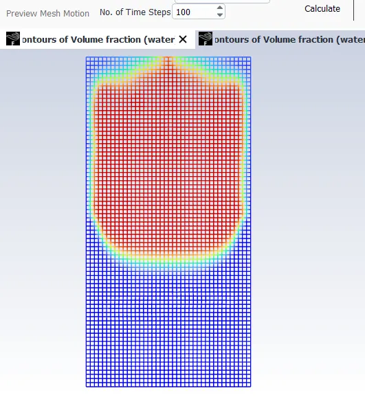
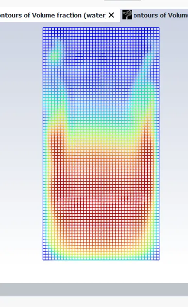
Change in contour plot phase wise:

One:

Two:

Three:

Four:

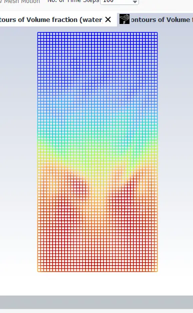
Final Contour plot:

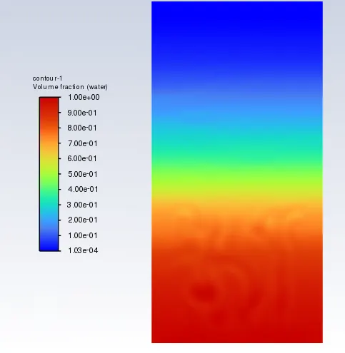
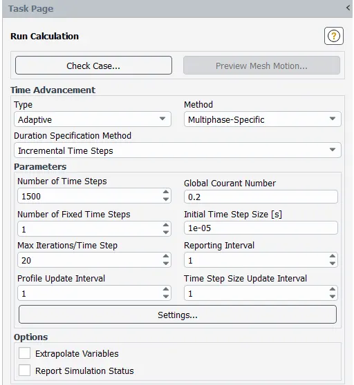
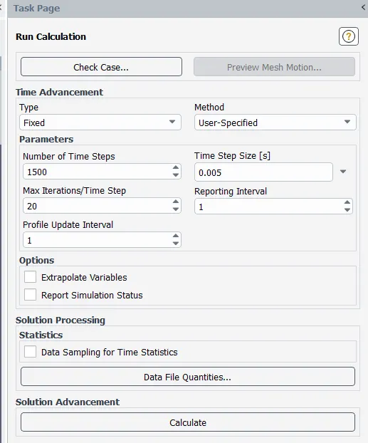
For more precise results, adaptive time step is used and simulation is performed but there is no deformation of the fluid layers. So fixed time step is again carried on by varying the global Courant number to 0.2 and the number of iteration is increased and the time step size is reduced to 0.005 and simulation is carried on.

Adaptive time step trial:

Fixed time step with modifications:

After initialization, calculation is done.

Viscous model: k-ω turbulance model

Type: Adaptive time step (trial)

Change in contour plot phase wise:

One:

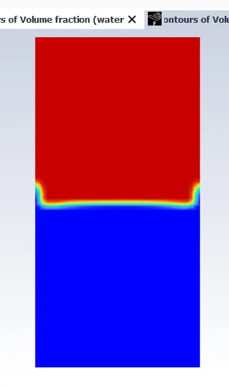
Two:

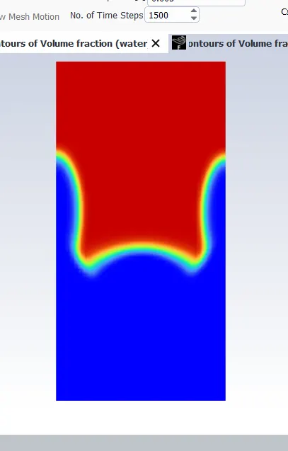
Three:

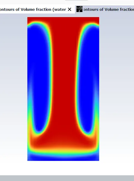
Four:

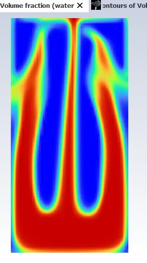
Five:

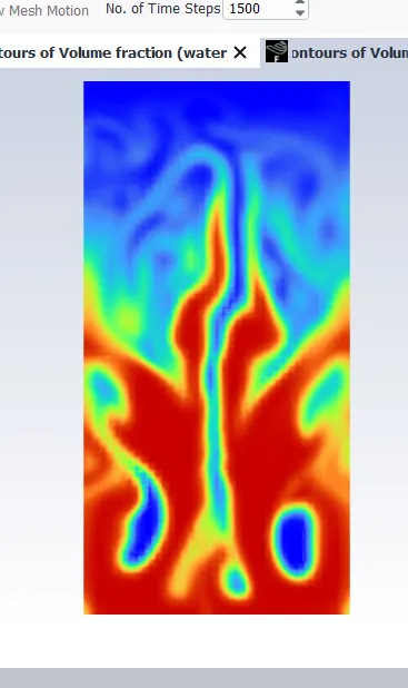
Six:

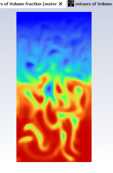
Seven:

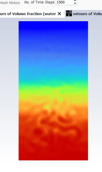
Final contour plot:

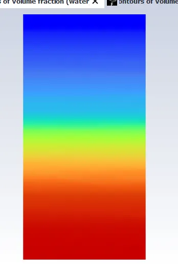
Case 2:

Mesh = 0.2 mm

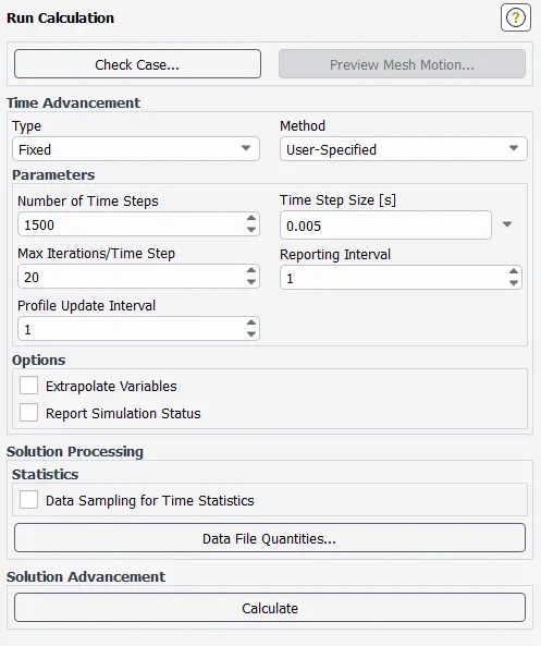
Type: Fixed time step

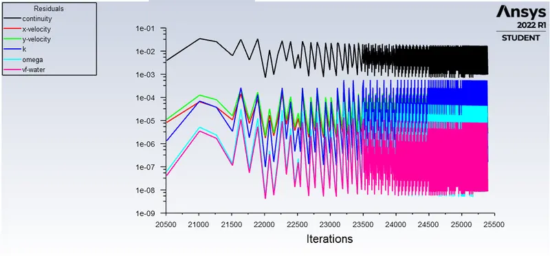
Scaled residuals:

Run calculation:

Change in contour plot phase wise:

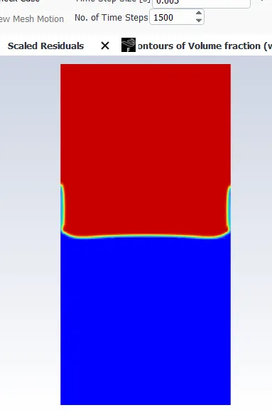
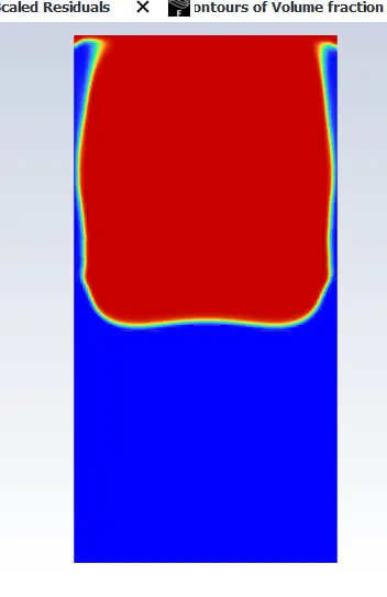
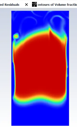
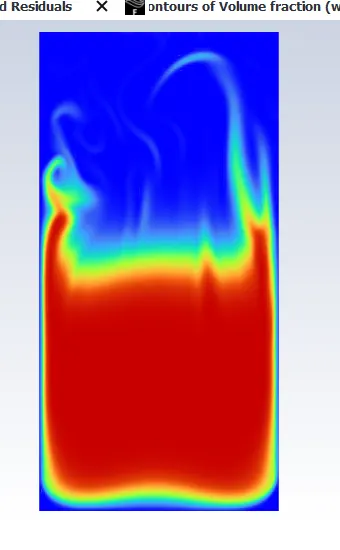
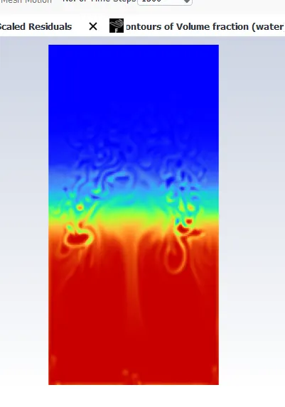
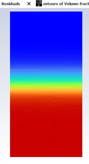
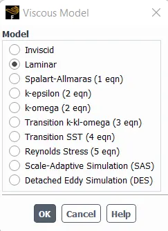
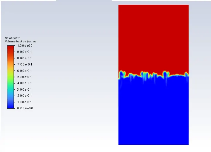
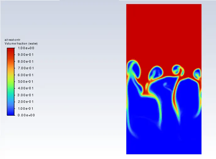
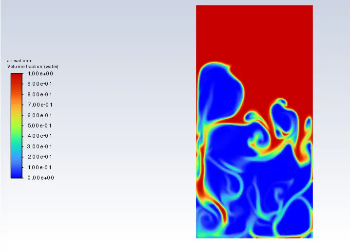
The above plot is made for turbulence model but we expect for laminar since the mixing is natural. So the correction has to be made for changing the viscous model to laminar and the number of iterations has to be reduced to 600 and time step size has to be reduced to 0.001.

Modified model contour plot phase change: (mesh =0.2)

1.

2.

3.

4.

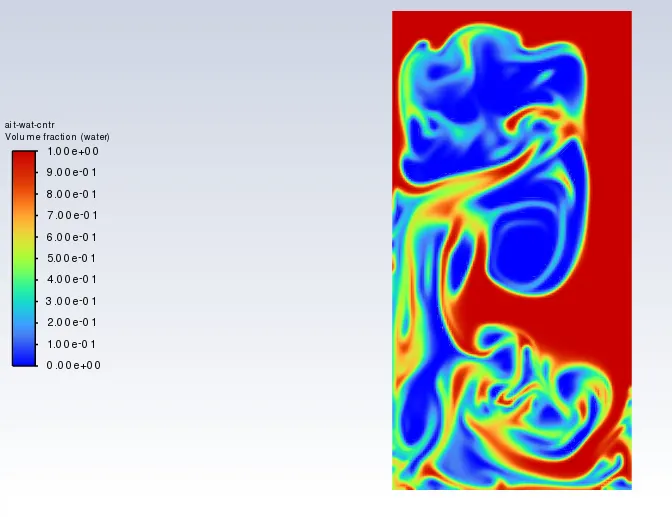
5.

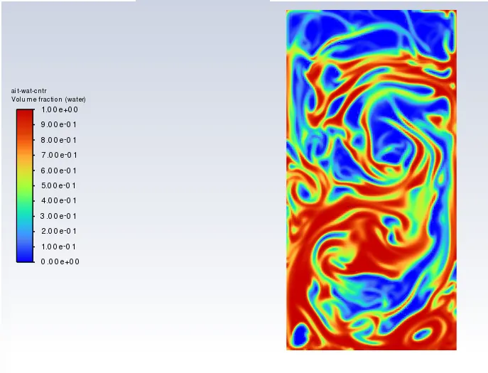
6. Final contour plot:

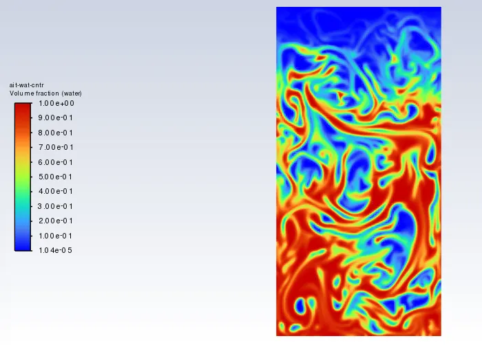
Video file link:

https://drive.google.com/file/d/1NECLBNiew0YcoCzZh68IZHXe-KJN_jb-/view?usp=sharing

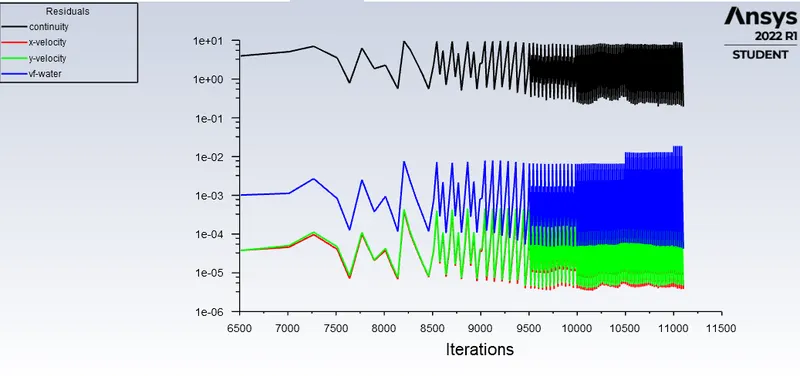
Residuals:

Case 3:

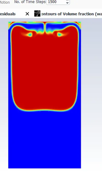
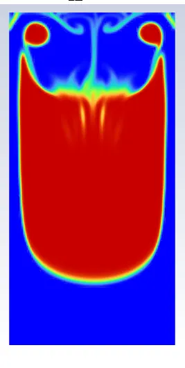
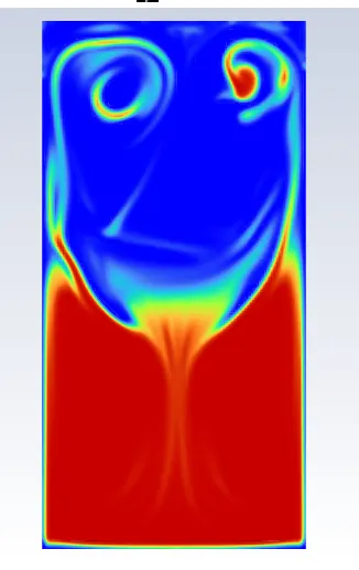
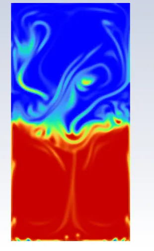
Water and user-defined material(density = 400 kg/m³, viscosity = 0.001 kg/m-s)

Primary phase: User defined material

Secondary phase: Water

Mesh = 0.2 mm

Viscous model: k-ω turbulance model

Phase One:

Phase two:

Phase three:

Phase four:

Phase five:

Phase six:

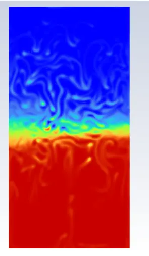
Final contour:

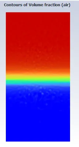
But the phase change behavior is not as expected as shown above. So this has to be corrected with Laminar flow model since the mixing of the fluid is natural and not forced one.

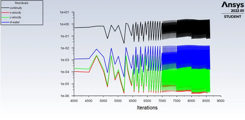
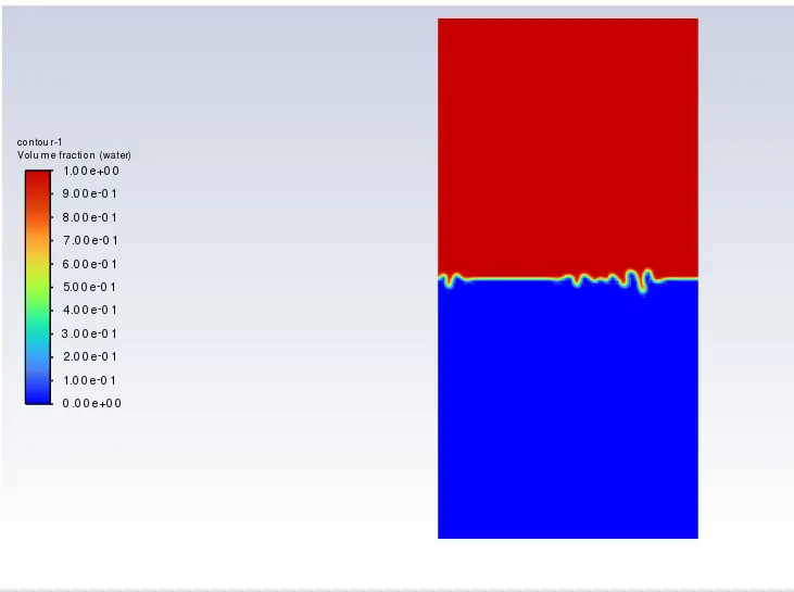
Rectified mixing model:

Viscous model: Laminar

No of iterations: 600

Time step size: 0.001

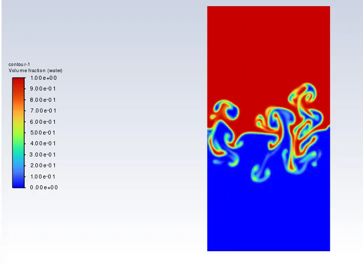
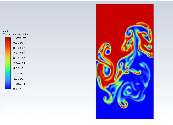
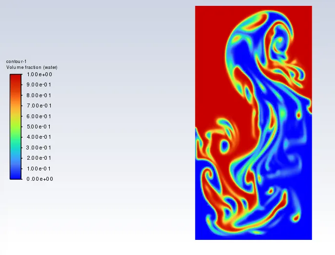
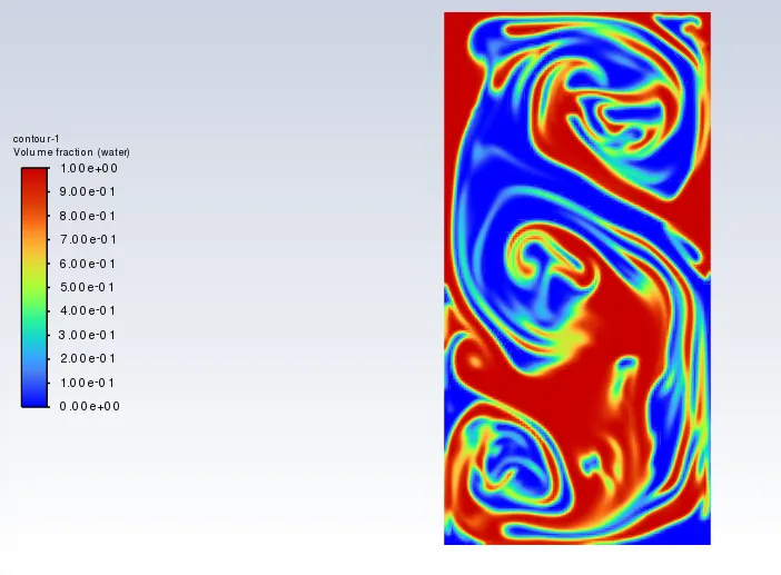
mesh = 0.2

Residuals plot:

Phase mixing contour plot:

Video file link:

https://drive.google.com/file/d/1WI6AE2C8ZQ0gsBe0lxiOX5kT296aslAi/view?usp=sharing

4. Define the Atwood Number. Find out the Atwood number for both the cases and explain how the variation in Atwood number in the above two cases affects the behavior of the instability.

The Atwood number is a dimensionless number in fluid dynamics used in the study of hydrodynamic instabilities in density-stratified flows. The Atwood number equals the ratio of the difference in mass densities to their sum.

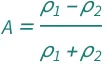
symbol	description	physical quantity
A	Atwood number	"AtwoodNumber"
ρ1	fluid density	"MassDensity"
ρ2	fluid density of lighter fluid	"MassDensity"

Case 1:

ρ1 = 1.225 kg/m^3

ρ2 = 998.2 kg/m^3

A = 0.9975

Case 2:

ρ1 = 400 kg/m^3

ρ2 = 998.2 kg/m^3

A = 0.4278

Atwood number is an important parameter in the study of Rayleigh–Taylor instability and Richtmyer–Meshkov instability. In Rayleigh–Taylor instability, the penetration distance of heavy fluid bubbles into the light fluid is a function of acceleration time scale.

WKT, F=ma

Therefore, a = F/m

where m = mass, which is proportional to density of the fluid.

So if the difference in densities of the fluids are more, the acceleration will be more and hence instability will be more at initial stage. Later, it will reach to equilibrium stage at faster rate. So the time taken to settle down will be less. In this case the splashing effect will be more in case of turbulance. It will lead to more asymmetrical pattern and accelerating leading to non-linear growth rate.

On the other hand, if the difference in the densities are less, the accelaration will be less and instability will be less. There will be gradual change in phase. Time taken to settle down will be more. The splashing effect will be less in case of turbulance model and we can observe near symmetrical pattern and accelerating leading to linear growth rate.

Reason for choosing Transient state instead of steady state approach:

In Rayleigh Taylor Instability simulation, we are interested in observing the flow pattern and phase change behavior of the two fluids at every time step. So transient simulation is chosen which the phase change is time bound behavior where as in Steady state simulation is time independent study. We need to observe the mixing pattern at each stage in which the transient simulation is suitable.

Steady state simulation is carried only when we are interested in the end result only and the mixing of fluid behavior is not necessary. But here, the simulation time will be less.

CONCLUSION:

• It is observed from the above experiment that when mesh gets finer, the mixing pattern and phase change are clearly observed at each iteration and time step.
• As the mesh size gets finer, the simulation time gets increased since more number of cells are there to perform simulation. So it is necessary to choose optimum mesh size.
• It is observed that as the Atwood number gets decreased, the acceleration rate varies linearly and the phase mixing is gradual and vice versa.
• In the mixing pattern bubbles formations are observed initially during mixing and disappears on later stage which leads to swirl pattern.