Rayleigh Taylor Instability

The Rayleigh-Taylor is an instability of an interface between two fluids of different densities which occurs when the lighter fluid is pushing the heavier fluid. A good example would be water suspended on oil, under the influence of earth's gravity.

As the RT instability develops, the initial perturbations progress from a linear growth phase into a non-linear growth phase, eventually developing "plumes" flowing upwards and "spikes" falling downwards.

There have been numerous CFD models based on the mathematical analysis of the RT instability. They are:

1. Mass diffusion model

2. Single Fluid Model:

1. Potential Flow model: The velocity is described as a gradient of any scalar function cause irrotation.
2. Buoyancy Drag model: based on ordinary differential equations, for estimating the growth of a turbulent mixing zone at an interface between fluids of different density due to Richtmyer–Meshkov and Rayleigh–Taylor instabilities

3. Multi Fluid model

In this project, a simulation of the rayleigh-Taylor Instability will be conducted in ANSYS using the FLUENT. The phenomenon observed during this instability will be seen in the simulation as well. The effect of changing the mesh size and changing the material will be simulated too.

Geometry

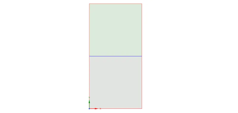
The simulation is a 2D simulation, and the geometry can be created in SpaceClaim. The geometry consists of two surfaces, stacked on top of each other on the XY plane. Each surface is a square of side length 20mm. The upper square is for the heavier fluid (water) and lower square is for the lighter fluid (air). The surfaces' topology is shared between them using the Share tool (under Workbench).

This is the final geometry from SpaceClaim:

Meshing

The default mesh with a sizing of 0.5mm was used for the base setup. The default mesh element shape is a square, which is the best fit for this type of simulation.

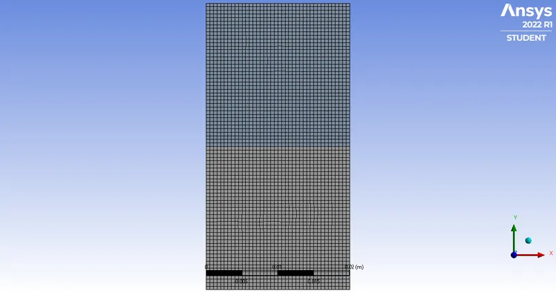
This mesh has 3200 elements and 3321 nodes.

This is the mesh metric for the base mesh:

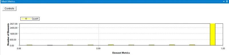
Almost all elements have a quality of 1 while a few have quality of 0.98 and 0.99. This quality is still greater than 0.7 so the mesh quality is satisfactory.

Simulation Setup

General

Solver: Pressure based, Transient and Planar

Gravity Enabled along the Y axis for a value of -9.81m/s2">m/s2�/�2

Models

Viscous - Laminar was the model used.

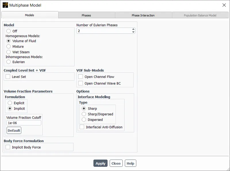
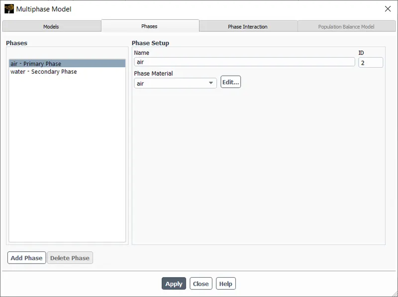
Multiphase -

Boundaries

All boundaries were left unchanged.

Materials

The existing materials' (air and water-liquid) properties were used and were left unchanged.

Density of Air: 1.225kg/m3">1.225kg/m31.225��/�3

Viscosity of Air: 1.7894⋅10-5kg/m.s">1.7894⋅10−5kg/m.s1.7894⋅10-5��/�.�

Density of Water: 998.2kg/m3">998.2kg/m3998.2��/�3

Viscosity of Water: 0.001003kg/m.s">0.001003kg/m.s0.001003��/�.�

Solution - Methods

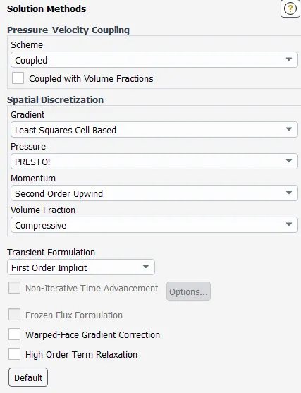
Contours were created for volume fraction of water throughout the entire surface. An animation was also created for the contour for every timestep.

The solution was initialised using the standard method. After every initialisation, the domain was patched using the patch tool for the following settings:

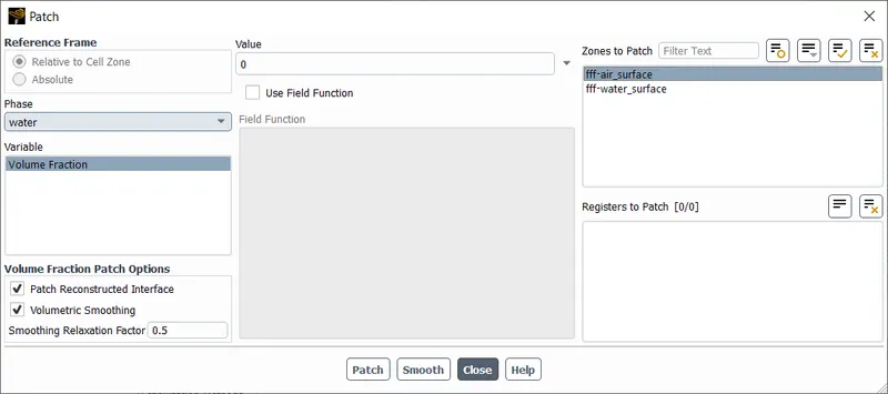
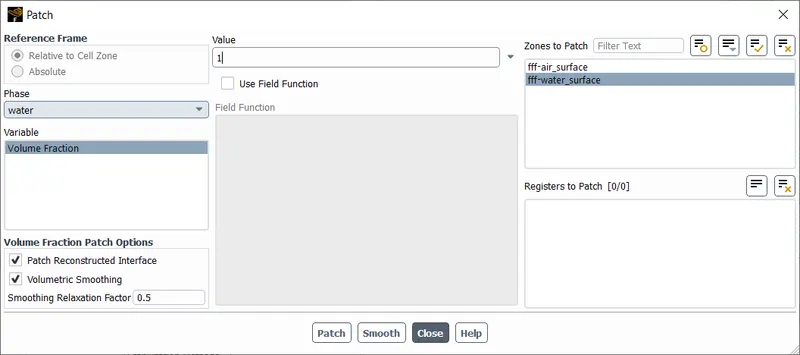
The solution was ran for 1000 timesteps, with each timestep being 0.005s long.

Simulation Results

The same settings were used for all simulations and the results are below, for each different grid size.

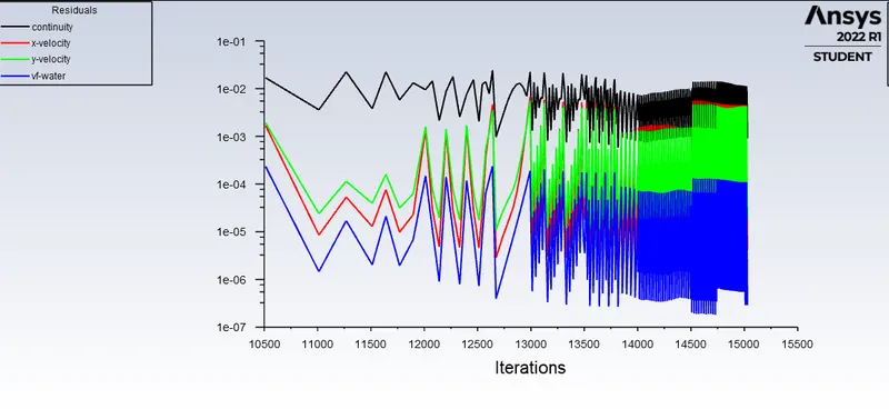
Base Setup (0.5mm grid size)

Residuals

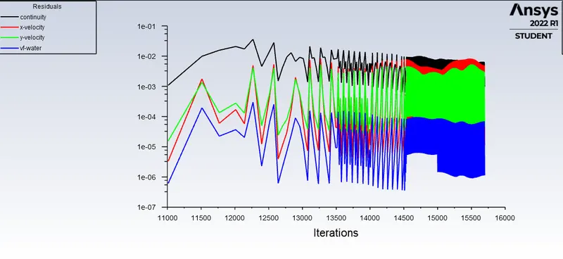
Coarser Grid Size (1mm)

Redisuals

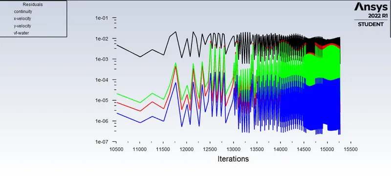
Finer Grid Size (0.25mm)

Residuals

User Definied Material

In this case, air was replaced with a user defined material of the following properties:

Density: 400kg/m3">400kg/m3400��/�3

Viscosity: 0.001kg/m.s">0.001kg/m.s0.001��/�.�

Other simulation parameters were the same.

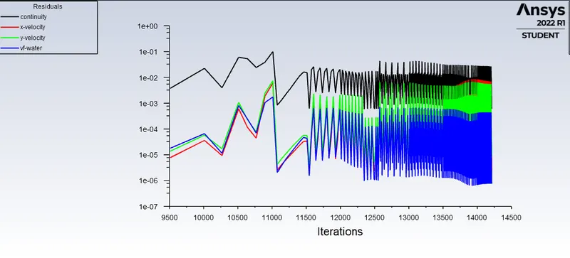
Residuals

The diffusion occuring in this simulation is slower than the ones before. This rate of diffusion can be quantified using the Atwood Number

The Atwood Number is a dimensionless number used in density stratified flows. It is the ratio of difference in densities of the fluids to the sum of the densities of the fluid. It is denoted by A">A� and given by:

A=ρ1-ρ2ρ1+ρ2">A=ρ1−ρ2ρ1+ρ2�=�1-�2�1+�2

where, ρ1">ρ1�1 and ρ2">ρ2�2 are densities of heavier and lighter fluid, respectively.

The acceleration of the heavier fluid particles into the lighter fluid is a function of A>2">A>2�>2 where g">g� is the gravitational acceleration and t">t� is the time.

For the air-water simulation, the Atwood Number is 0.99.

For the user_material-water simulation, the Atwood Number is 0.42.

The higher the Atwood Number, the more prominent huge bubbles of fluid are in the simulation.

Conclusions and Observations

1. The simulation runs well and its results are consistent with expected results and experimental data.

2. Increasing the Grid Size results in a more coarse animation, the bubbles are not as clearly visible. The gradient between the fluids is less in a coarse grid (the transition from one fluid to another is sudden and not gradual).

3. Minor movements of the fluid particles are also not visible when the grid size is decreased. Overall, decreasing the grid size provides for a such more smoother looking animation and an animation that closely resemebles experimental results.

4. Swapping air for a user defined material of higher density than air decreases the acceleration of the heavier fluid into the lighter fluid. This can and is quantified by the Atwood Number, which was mentioned in the report.