Week 5 - Rayleigh Taylor Instability

REPORT FOR CHALLENGE-5

Aim : To simulate and visualize the Rayleigh Taylor instability while interacting one fluid with another for the two cases of different mesh cases.

Software Required : Ansys Workbench – Fluid Flow vR2-2022

Hardware Required : Desktop, Keyboard, Mouse, CPU.

Theory:

Rayleigh–Taylor instability (or RT instability) is named after Lord Rayleigh and G. I. Taylor. There are situations where a heavy liquid layer is placed over a lighter fluid layer. This situation has engineering implications in several industries. For example in die casting, liquid metal is injected in a cavity filled with air. In poor designs or other situations, some air is not evacuated and stay in small cavity on the edges of the shape to be casted. Thus, it can create a situation where the liquid metal is above the air but cannot penetrate into the cavity because of instability. This instability deals with a dense, heavy fluid that is being placed above a lighter fluid in a gravity field perpendicular to interface.

Example for such systems are dense water over oil (liquid–liquid), or water over air(gas–liquid). The original Rayleigh's paper deals with the dynamics and density variations. For example, density variations according to the bulk modulus are always stable but unstable of the density is in the reversed order. Supposed that a liquid density is arbitrary function of the height. This distortion can be as a result of heavy fluid above the lighter liquid. This analysis asks the question of what happen when a small amount of liquid from the above layer enter into the lower layer? Whether this liquid continue and will grow or will it return to its original conditions? The surface tension is the opposite mechanism that will returns the liquid to its original place. This analysis is referred to the case of infinite or very largeer surface.

The simplified case is the two different uniform densities. For example a heavy fluid density , ρL">ρL, above lower fluid with lower density, ρG">ρG. For perfectly straight interface, the heavy fluid will stay above the lighter fluid. If the surface will be disturbed, some of heavy liquid moves down. This disturbance can grow or returned to its original situation. This condition is determined by competing forces, the surface density, and the buoyancy forces. The fluid above the depression is in equilibrium with the sounding pressure since the material is extending to infinity. Thus, the force that acting to get the above fluid down is the buoyancy force of the fluid in the depression.

The depression is returned to its original position if the surface forces are large enough. In that case, this situation is considered to be stable. On the other hand, if the surface forces (surface tension) are not sufficient, the situation is unstable and the heavy liquid enters into the liquid fluid zone and vice versa. As usual there is the neutral stable when the forces are equal. Any continues function can be expanded in series of cosines. Thus, example of a cosine function will be examined.

Atwood number: It is a dimensionless number in fluid dynamics used in the study of hydrodynamic instabilities in density stratified flows. It is a dimensionless density ratio defined as

                 A=ρ1-ρ2ρ1+ρ2">A=ρ1−ρ2 /A=ρ1-ρ2ρ1+ρ2">ρ1+ρ2

where,

ρ1 = density of heavier fluid

ρ2 = density of lighter fluid

 -More the atwood number, more the instability and less the atwood number more the stability.

Procedure :

• Geometry:

1. Open the space claim.
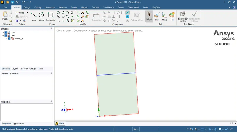
2. Draw a square with 20 by 20 mm and make it as a surface then change it to a new component and name it as air.
3. Then again draw another square of length 20 by 20 mm on the top of the drawn square and make it as a new surface and name it as a water
4. Then do the top-share in workbench section for to assign the common node points while meshing.

• Meshing:

1. Open meshing.
2. Select the element size and apply mesh on the geometry(5mm and 3mm).
3. Select the lower surface for the name of selection and name it as air.
4. Then again select the upper surface and name it as water.

• Set-up and solving:

1. Open setup by choosing the requirements of your laptop for the solving process.
2. Change solver to transient and set the gravity in the direction of y with -9.81.
3. Set the k-Omega or laminar model in the viscous section.
4. Now open the materials and assign the air and water as fluids.
5. Select the multiphase and change to volume of fluid method then change explicit to implicit.
6. Now assign air as the primary phase and water as the secondary phase.
7. Open the solution section and initialise.
8. Now open the patching and change mixture to water, select the volume of fluid and assign the water with the volume fraction of 1, patch and close.
9. Now create a solution animation file for the created contour.
10. Then enter the perfect time step size and number of time steps, calculate.
11. After solving all the equations, save the animation file in the video format.
12. Then save the project and close the work bench.

Observations :

Geometry:

-Model to be Analized.

 

Mesh Details:

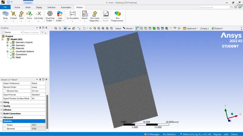
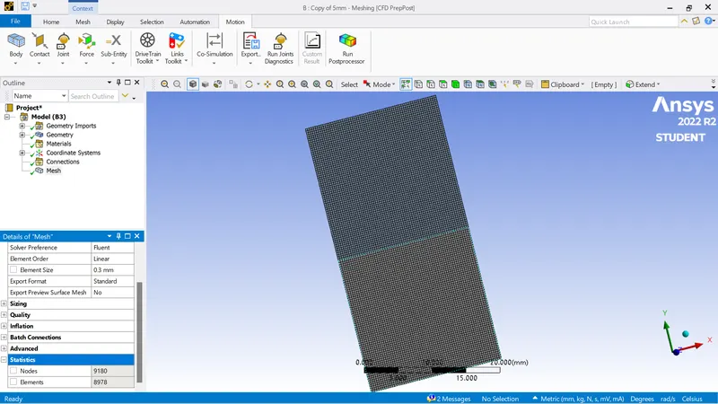
On the consideration of the accuracy of the result, we worked on the concept of independent grid generation. So, we analysed the given exhaust port in 2 different cases which are Medium and Fine mesh and all the mesh details were given below,

Mesh	Size	No.of elements
Medium	5mm	3200
Fine	3mm	8978

1.Medium Mesh:

 

2.Fine Mesh:

 

Material Settings:

Fluid	1.Air
	2.Water

General Settings:

• Gravity - -9.81 m/s^2
• Solver - Transient

Physics Settings:

-Multi-Phase:

• Volume of fluid
• Implicit
• 2 Phases

1. Primary - Air
2. Secondary - Water

Solution Settings:

-Patching:

• Water with volume fraction of 1.

Case-1:

-Simulation is run with - Time Step Size = 0.005 & No. of Time Steps =1200

Plots and Contours:

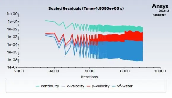
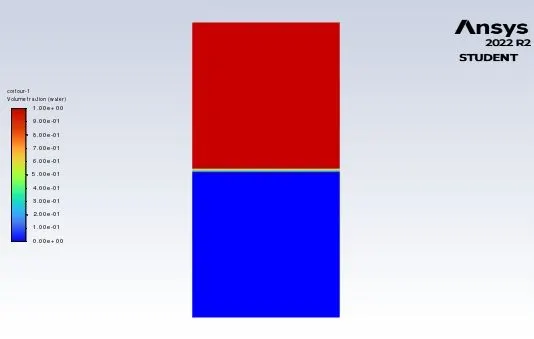
Volume Fraction contour after patching water with 1.

Case-2:

-Simulation is run with - Time Step Size = 0.005 & No. of Time Steps =1000

Plots and Contours:

 

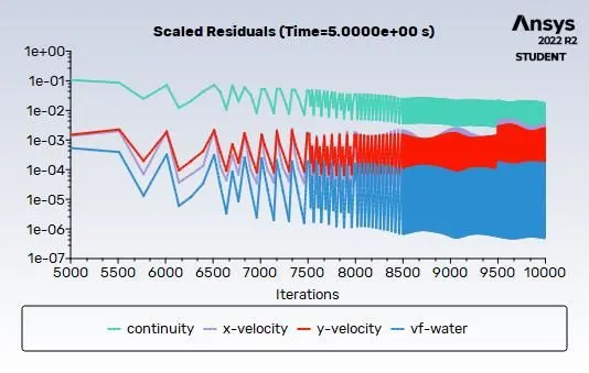
Volume Fraction contour after patching water with 1.

Precautions :

1.Carefully solve the problem.

2.Choose the suitable methods carefully for to get the desired results.

3.Note down the values carefully which are required for theoretical calculations.

Result:

• Atwood number=0.9975

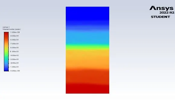
case-1:

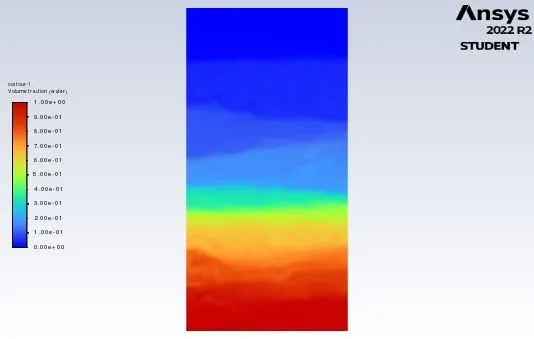
case-2:

 

Conclusion:

Rayleigh Taylor instability was observed at the interface of the fluids with different density under the influence of gravity. The lower density fluid pushes the higher density fluid above it. The heavier fluid which is water, in this case, comes at the bottom and replaces the air from the bottom. The formation of air bubbles takes place which moves upward. The mesh refinement leads to better simulation of the Rayleigh Taylor instability. All the instability and the irregularities that take place at the interface are better visualized as we refined the mesh.

The steady-state analysis is used when we are more concerned with the end result. But for Rayleigh Taylor instability we are more interested in observing the real-time changes of the interface and the fluid region. The real-time observation is possible only in Transient State analysis.

After performing the 2 different case setups with respect to grid sizes, we can conclude that the finer the mesh the greater the possibility of accurate flow prediction.