Week 5 - Rayleigh Taylor Instability

Aim: Study of Rayleigh Taylor instability

Objectives:

• To understand and set up multiphase fluid flow problems without fluid interactions.
• To understand the instability associated with the mixing of fluids at different densities.
• To understand and evaluate the extent and behaviour of this mixing with the help of a dimensional number (Atwood number)
• To understand the effect of fluid properties on the behaviour of instability.

Introduction:

The Rayleigh Taylor Instability (RTI) is observed at the interface of two immiscible fluids when the fluid of higher density gushes through the fluid at a lower density and thereby mixing occurs under the influence of gravity. This is a complex and dynamic process wherein the fluid system aims at minimisation of the combined potential energy of the fluids present in the system. Some notable examples of this phenomenon could be the mixing of oil and water, mushroom cloud formation from high-energy explosives or volcanic eruptions, or molten metal poured into the sand casting.

There exist some practical CFD models based on the RTI phenomenon which are discussed below:

1. Kelvin Helmholtz Instability
   This model provides the prediction of transition to turbulent flow in fluids of different densities exhibiting a relative motion above their interface. The discontinuity at this interface of the fluid generates shear stress which leads to the formation of an unstable vortex sheet that propagates in the form of a spiral. For example, the waves formed over the surface of water bodies by wind blowing over the surface.
2. Richtmyer Meshkov Instability
   This model is applicable to cases wherein two fluids of different densities are accelerated impulsively by the passage of shock waves and thus leading to instability. The onset of this instability is experienced by small perturbations (disturbance) which grow initially linearly with time, which is consequently followed by a non-linear regime with bubble formation in cases where lighter fluid penetrates the heavy fluid and spikes in case the heavy fluid penetrates in the lighter fluid.
3. Plateau Rayleigh Instability
   This model explains why and how the falling stream of fluid breaks into packets of the same volume but lesser surface area. The principle behind this is that fluids tend to minimise its surface area owing to the effect of surface tension. This instability can be seen in case of a liquid jet emerging from a pipe or hose breaks into large droplets.
4. Saffman Taylor Instability
   Also known as viscous fingering, it is the formation of patterns in a morphologically unstable interface between two fluids in a porous medium. It occurs when a less viscous fluid is injected, displacing a more viscous fluid; in the inverse situation, with the more viscous displacing the other, the interface is stable and no instability is seen.

Workflow:

1. Preparing the geometry
2. Generate mesh for the geometry
3. Setting up the solver
4. Setting up the solution monitors
5. Post-processing to observe the results

Ansys Fluent:

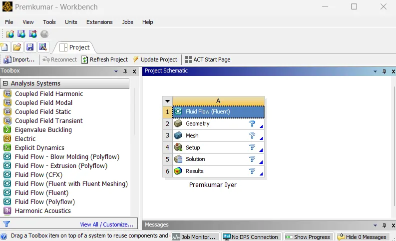In the Ansys workbench project window, Fluid Flow (Fluent) is dropped into the workspace.

Preparing the geometry:

The computational domain followed for the simulation is as shown below:

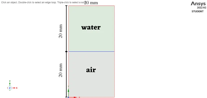The computational domain, as shown is created in SpaceClaim. New components are introduced in the structure tree for air and water respectively. The 2D sketch for the air region is drawn and on escaping the sketch plane, the closed loop forms a surface. Similar work is done for the water region. These different components created help to ease the "patching" which will be discussed subsequently. To generate a conformal mesh, the common edge needs to be shared and this is done by sharing the topology between the two components. Thus the common edge, upon detection by the share prep tool under the workbench tab is shared. And hence, the geometry is created.

Generating mesh:

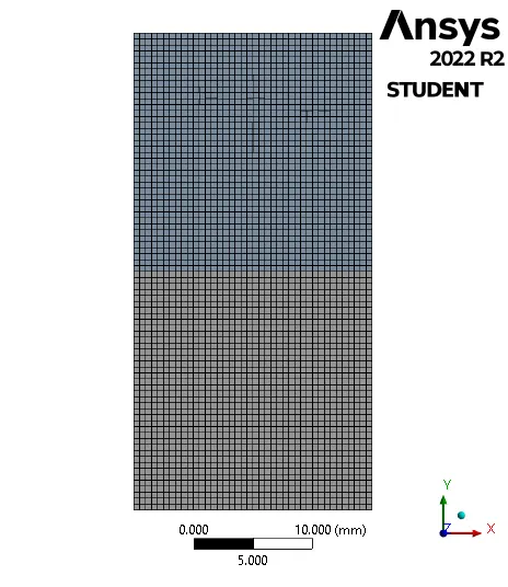
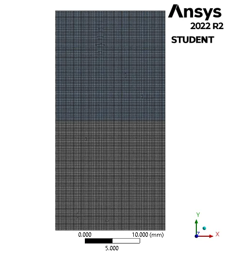
Meshing is the process, wherein the geometry is divided into smaller parts which are known as elements so that the iterative solver can solve the governing equations across the domain. In the meshing utility, a baseline mesh of element size 0.5mm is provided. Since we study the effect of mesh size on the simulation, we have the following meshes:

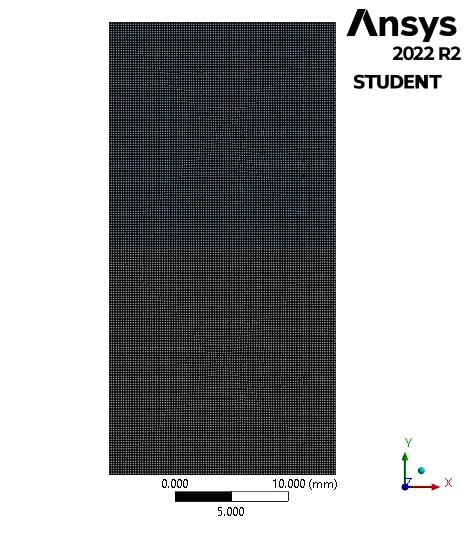Mesh-1 (Element Size: 0.5mm; No. of Elements: 3200)	Mesh-2 (Element Size: 0.25mm; No. of Elements: 12800)	Mesh-3 (Element Size: 0.15mm; No. of Elements: 35378)

Since, the case does not involve any fluid inflow or outflow, the mesh inputs (such as methods, sizing or inflation) are not provided. The effect of the above mesh element size change is observed.

Setting up the solver:

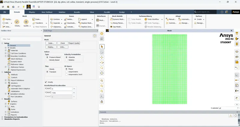An important part of a CFD simulation, the setup for solver is done to obtain the solution. Firstly, the units of important parameters are set to desired units (preferably SI units). Since the problem is of multiphase fluid flow, the model with volume of fluid (VOF) in the implicit formulation is implemented. The material properties for air and water are imported from the fluent database. Then, in the multiphase tab, the phases are defined, with air being the primary phase and water as the secondary phase. In the viscous models, laminar is chosen (and it will take care of the vigorous mixing of the air and water). Boundary conditions need not be provided.

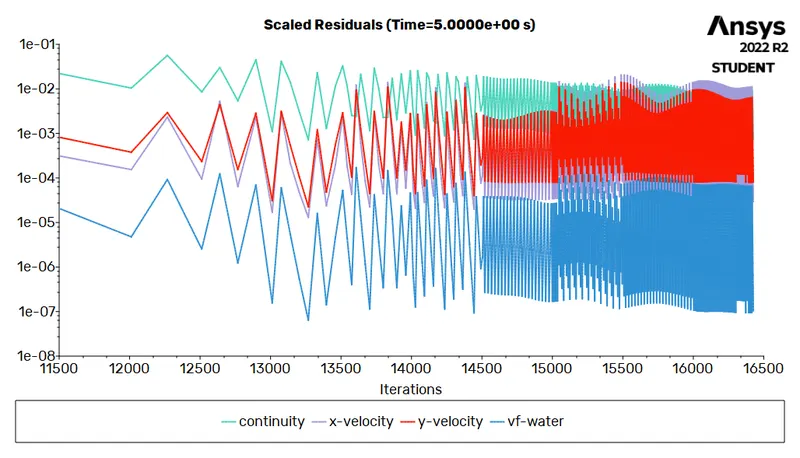
The pressure-velocity coupling is set to SIMPLE and the gradient is least squares cell-based, the momentum in second-order, pressure as PRESTO!, volume fraction as compressive and implicit formulation in first-order discretisation. The case is initialised with hybrid initialisation, and the air region and water region are patched with respect to the volume fraction of water (1 in water region and 0 in air region). The contour of water volume fraction is created to check this. Under the solutions tab, the solution animation for this contour is created to capture changes in the contour for every time step. The calculations are run by fixed time advancement, 0.005sec of time step, 20 iterations per time step and 1000 number of time steps (therefore a flow time of 5sec).

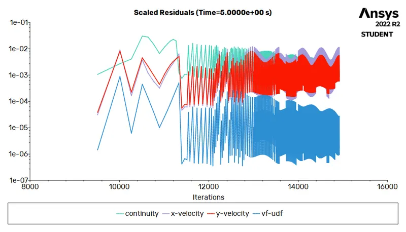
The same case is studied by replacing water with a user-defined fluid with density of `400 kg//m^3` and viscosity of `0.001 Pa-s`.

Post-processing (Results):

The results for water and air:

Mesh-1	Mesh-2	Mesh-3

The results for the user-defined fluid and air:

Conclusion:

• In this instability problem, mixing was studied and the effect of mesh size was observed. The bubbles of water rises and water, being of higher density (than air) settles down. With refinement in mesh size, the dynamics of instability becomes clearer, such as the random motion within the water after it settles, the splashing of water as strikes the bottom and the edges, and the rise of minuscule air bubbles that were trapped when water pushed through it.
• Atwood number is a dimensionless number that describes the density difference between two fluids sharing the same interface which characterise the hydrodynamic instability in density stratified flows.
  Atwood number ` (A) = (rho_1 - rho_2) / (rho_1 + rho_2)`
  where, `rho_1` is the denser fluid and `rho_2` is the lighter fluid.
  
  1. Water and air:
     The density of water and air is 998.2 and 1.225 `kg//m^3` respectively, therefore
     `A = (998.2 - 1.225) / (998.2 + 1.225) = 0.9975`
  2. User defined fluid and air
     The density of the fluid and air is 400 and 1.225 `kg//m^3` respectively, therefore
     `A = (400 - 1.225) / (400 + 1.225) = 0.9939`
• The Atwood number provides a good prediction of penetration of denser fluid into a lighter fluid (with time as `A g t^2`, where `A` is the Atwood number, `g` is acceleration due to gravity and `t` is the time). For lower Atwood number, the lighter fluid fluid rises in the form of fringes (due to similarity on densities) and for higher Atwood number the lighter fluid rises in the form of huge bubble like cloud structure due larger density difference.
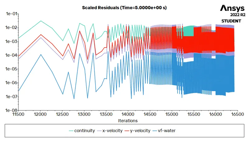
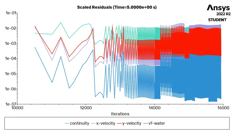
• Although the problem is of unsteady nature and cannot be solved by steady state solver, but when solution is forced in steady state it behaves erratically. The fluid exhibits a weird motion and the solver abruptly stops stating floating point exception.
  
• Therefore, study on Rayleigh Taylor instability is done successfully.

References:

• Introduction to GUI based CFD using Ansys Fluent - Course provided by Skill Lync.
• Ansys Inc.
• Supporting Material: Rayleigh-Taylor Instability: Scholarpedia
• Supporting Material: LibreText: Rayleigh Taylor Instability
• Supporting Material: The Rayleigh–Taylor instability in a porous medium
• Supporting Material: A Drop of Science: Rayleigh Taylor Instability