Week 5 - Rayleigh Taylor Instability

week 5 challenge::

aim:

to perform a rayleigh taylor instability simulation and analyse the results.

introduction:

free surface flow are successfully modelled with one of the existing free flow surface model.the most commonly used model methods are level set method and volume of fluid method.beside this model there are so many models are used.

free surface flow is also called as open channel flow. the gravity driven flow of a fluid under a free surface typically water flowing under air or atmosphere.

Level-set methods (LSM) are a conceptual framework for using level sets as a tool for numerical analysis of surfaces and shapes. The advantage of the level-set model is that one can perform numerical computations involving curves and surfaces on a fixed cartesian grid without having to parameterize these objects (this is called the Eulerian approach). Also, the level-set method makes it very easy to follow shapes that change topology, for example, when a shape splits in two, develops holes, or the reverse of these operations. All these make the level-set method a great tool for modeling time-varying objects, like inflation of an airbags, or a drop of oil floating in water.

The underlying technology is called the ‘Volume of Fluid’ (VOF) method. In the case of air and water, this assigns a volume fraction of air and water to each cell in the domain. The sum of the two fractions is always 1, so calculating one fraction always implies the other. Where the volume fraction is 0.5, there will be a free surface. Either side of this cell the volume fraction will tend towards fully water or fully air. As with all Flow simulations, the software calculates the mass and volume of fluids entering and leaving each cell and conserves momentum, energy and mass. However, the actual movement of the free surface is obtained using ‘transport equations’ driven by fluid momentum calculations and external boundary conditions including gravity. More details are available in the Flow Simulation Technical Reference.

rayleigh taylor instablity:

The Rayleigh–Taylor instability, or RT instability (after Lord Rayleigh and G. I. Taylor), is the instability of an interface between two fluids of different densities which occurs when the lighter fluid is pushing the heavier fluid. Examples include the behavior of water suspended above oil in the gravity of earth, mushroom clouds like those from volcanic eruptions and atmospheric nuclear explosions, etc.

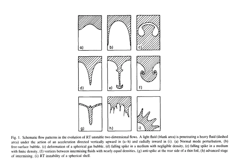
figure shos the RT instablity.

the RTI consists of four stages they are:

In the first stage, the perturbation amplitudes are small when compared to their wavelengths, the equations of motion can be linearized, resulting in exponential instability growth. In the early portion of this stage, a sinusoidal initial perturbation retains its sinusoidal shape.

However, after the end of this first stage, when non-linear effects begin to appear, one observes the beginnings of the formation of the ubiquitous mushroom-shaped spikes (fluid structures of heavy fluid growing into light fluid) and bubbles (fluid structures of light fluid growing into heavy fluid). The growth of the mushroom structures continues in the second stage and can be modeled using buoyancy drag models, resulting in a growth rate that is approximately constant in time. At this point, nonlinear terms in the equations of motion can no longer be ignored

The spikes and bubbles then begin to interact with one another in the third stage. Bubble merging takes place, where the nonlinear interaction of mode coupling acts to combine smaller spikes and bubbles to produce larger ones. Also, bubble competition takes places, where spikes and bubbles of smaller wavelength that have become saturated are enveloped by larger ones that have not yet saturated.

This eventually develops into a region of turbulent mixing, which is the fourth and final stage in the evolution. It is generally assumed that the mixing region that finally develops is self-similar and turbulent, provided that the Reynolds number is sufficiently large

mathematical approach of RTI:

Linear stability analysis

The inviscid two-dimensional Rayleigh–Taylor (RT) instability provides an excellent springboard into the mathematical study of stability because of the simple nature of the base state. This is the equilibrium state that exists before any perturbation is added to the system, and is described by the mean velocity field U ( x , z ) = W ( x , z ) = 0 , where the gravitational field is g = − g z ^ . An interface at z = 0 separates the fluids of densities , ρ G in the upper region, and ρ L in the lower region. In this section it is shown that when the heavy fluid sits on top, the growth of a small perturbation at the interface is exponential, and takes place at the rate.

exp ⁡ ( γ t ) , with γ = A g α and A = ρ heavy − ρ light ρ heavy + ρ light ,

where γ is the temporal growth rate, α is the spatial wavenumber and A is the atwood number.

CFD simulation:

pre processing:

first we have to open ansys workbench, then create a new project and save it.

then from the analysis system pick fluid flow (fluent model).drag and drop on project schematic.

the double click on geomentry. it open the space claim.

in that space claim draw a two rectangle and name the above rectangle as water surface and below as air surface.

then by using share . share the edges of the two rectangle.

these are shown in the below.

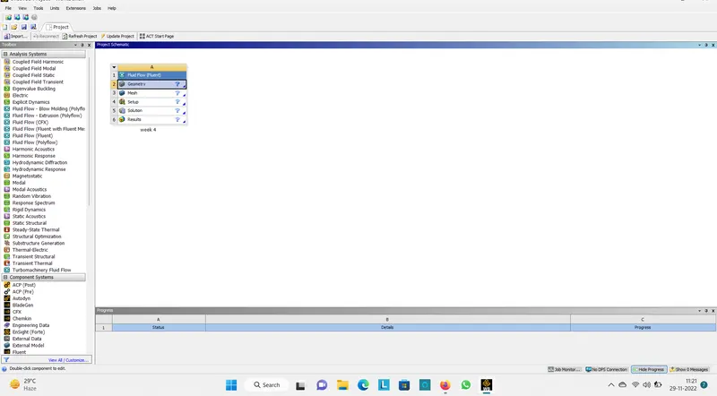
this is the fluid flow system.

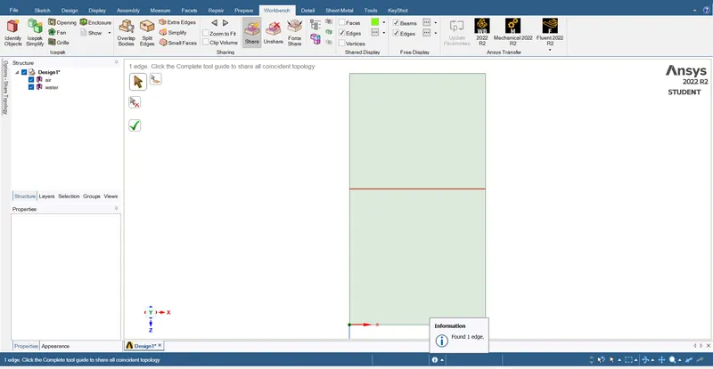
here the two surfaces are drawn and shared.

here then close the space claim window.

now double click on mesh in fluid flow system to open the mesh.

then create a mesh by right click on the mesh and generate mesh.

case1:

now base size of o.5mm is created by changing the element size.

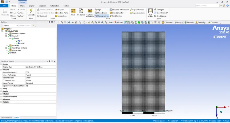
then we want to check the number of nodes, elements and the quality of mesh:

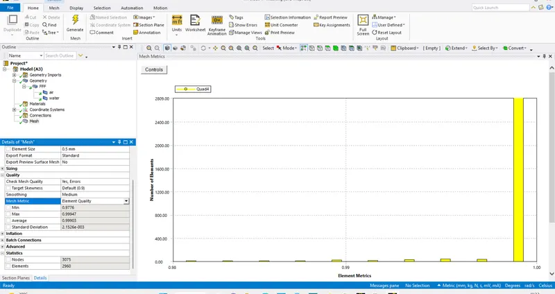
now close the mesh window. the creation of mesh is completed for case 1.

case2:

refined mesh1.

with the element size of 0.25mm.

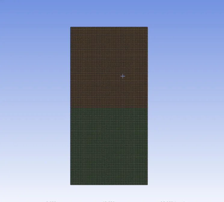
where the number of nodes, elements and the quality of mesh:

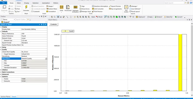
case3:

now base size of o.5mm is created by changing the element size.

then we want to check the number of nodes, elements and the quality of mesh:

processing:

then double click on setup in the system to open the fluent lauchetr.

here we use a double precision,parallel and 4 solver processes and click on start as shown in the below.

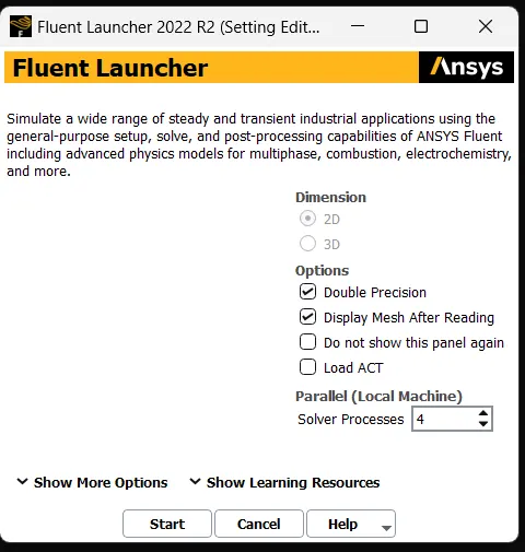
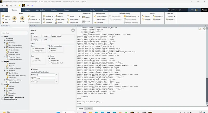
now we have first check for mesh quality.

then , pressure base solver type and the time is transient. with gravity enabled in -y direction with 9.81m/s^2

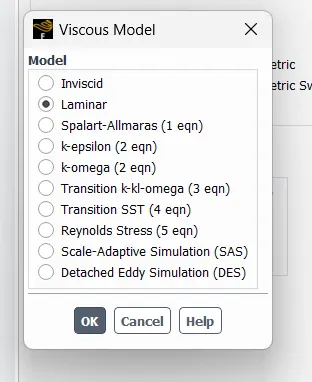
then for viscous is laminar model is chosen

then click on materials to get the materils as air and water.

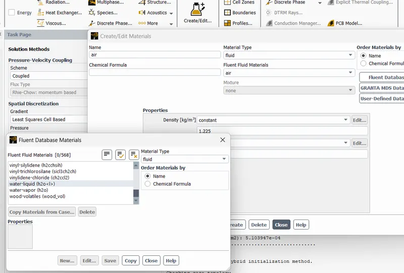
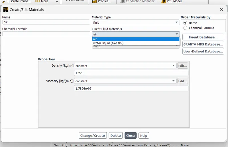
note::for case 4 only we have to modify the material by creating a user defined material with density 400kg/m^3,viscosity of 0.001kg/ms.

boundary condition are as:

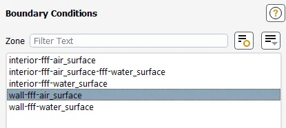
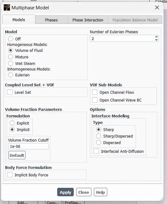
then click on multiphase. because we are using two phases in this model.

click on volume of fluids and implicit and click on apply.

then close the multiphase model dialog box.

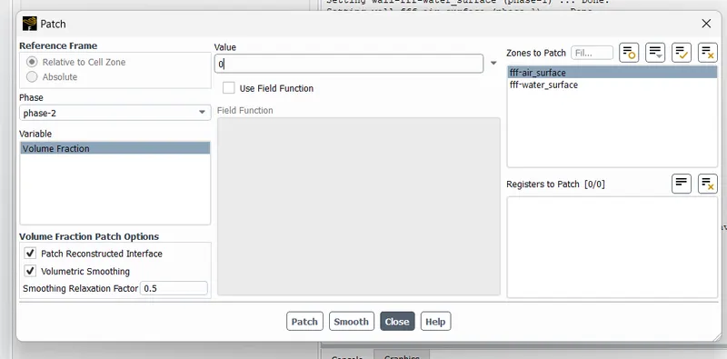
after multiphase initialize the model. then click on patch.

here in phase we want to chose phase 2. and in variable chose volume fraction.

then for the air surface value is 0 and for water surface value as 1. click patch indiviually we have to patch it.

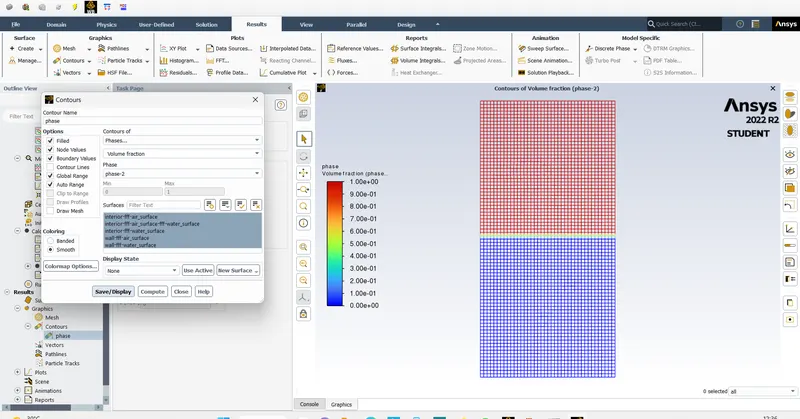
then go to reults>contour> create a contour of phase > save and display.

here we also needed to create animation video. for that in solution click on create animation.

post processing::

there are two ways to run the system.

one is the fixed time step variable with time step of 0.005 sec and the total time of 700 sec.

second one is adaptive time step method, where courant number is 0.2 and the maximum time variable of 0.05 and it runs upto 700 sec.

chose either one of the method and hit calculate.

after the code is run completely.now we have to download the animation and then we have to attach in the week 4 challenge.

the simulation are shown below.:

case1:

https://drive.google.com/file/d/1c6x_ubeTF36FT2ZhocuFNe11jV_T2YHD/view?usp=sharing

case2::

https://drive.google.com/file/d/1pYDHfzZhl8vtHNgmsj1VTmdKLkTcOqTI/view?usp=sharing

case3::

https://drive.google.com/file/d/1cPiqlTfTFYv20wSkuBl0-wTEk81MnMVn/view?usp=sharing

Atwood Number

It is a dimensionless number that is used to study hydrodynamic instabilities in density stratified flows.

A=ρ1−ρ2/(ρ1+ρ2)

Where,

ρ1

is density of heavier fluid

ρ2

is density of lighter fluid

For Air-water RT instability,

ρ1

= 998.2 kgm3">kg/m3

[Water density]

ρ2

= 1.225 kgm3">kg/m3

[Air density]

A = (998.2-1.225)/(998.2+1.225)

A = 0.998

For water- UD material RT instability,

ρ1

= 998.2 kgm3">kg/m3

[Water density]

ρ2

= 1.225 kgm3">kg/m3

[UD material density]

A = (998.2-400)/(998.2+400)

A = 0.428

a dimensionless number in fluid dynamics used in the study of hydrodynamic instabilities in density-stratified flows. here if the atwood number is increse the instabilities of the fluid increase and vice versa.

atwood number forms a basis to compare and study research papers based on RT Instabilty. Thus we can use these papers to validate our results for better accuracy.

conclusion:

simulation of the rayleigh taylor instability has been performed.

for different mesh the time for simulation varies and the refinement mash shows the detailed view of the rti.

for different density fluid the formation of the rti differs its shown by atwood number. where a atwwod close to 0 gives us a symmertric finger like shape.

for close to1 it gives us a larger bubble like plume shape in the flow.

referance::

https://sci-hub.hkvisa.net/10.1115/fedsm2008-55063

https://en.wikipedia.org/wiki/Rayleigh%E2%80%93Taylor_instability

https://sci-hub.hkvisa.net/10.1115/fedsm2008-55063

https://sci-hub.hkvisa.net/10.1016/B978-0-12-815485-4.00018-8