Week 5 - Rayleigh Taylor Instability

WEEK 5 CHALLENGE: DETAILED REPORT

Objective

1. What are some practical CFD models that have been based on the mathematical analysis of Rayleigh Taylor waves? In your own words, explain how these mathematical models have been adapted for CFD calculations.
2. Perform the Rayleigh Taylor instability simulation for 2 different mesh sizes with the base mesh being 0.5 mm. Compare the results by showing the animations( Attach them from your google drive). Observe the differences in the animation and explain the effect of mesh size on simulation. Also, explain why a steady-state approach might not be suitable for these types of simulation.[ Choose Air and Water for this simulation]
3. Run one more simulation with water and user-defined material(density = 400 kg/m³, viscosity = 0.001 kg/m-s) for refined mesh.
4. Define the Atwood Number. Find out the Atwood number for both the cases and explain how the variation in Atwood number in the above two cases affects the behavior of the instability.

Introduction

Fluid instabilities show up everywhere in nature. Fluid flow will start off laminar and smooth and then quickly transition to an irregular pattern eventually transitioning to turbulence.

Stratified fluid instabilities

From a fluid instability perspective, stratified fluid systems are in some ways the easiest to understand and visualize. It is often the case when there is a fluid system in which two fluids with different properties, an unstable configuration can be realized. In this case, there is a clear boundary between two fluids and this can be extended to a continuous variation between fluids, but the diffusion effects would damp out any perturbation and instability, so would not be as pronounced.

Buoyancy driven instabilities

Buoyancy-driven fluid instabilities occur in a stratified fluid system when the light fluid is accelerated into the heavier one often by means of a pressure gradient.

Some practical CFD models that have been based on the mathematical analysis of Rayleigh Taylor waves are:

Kelvin-Helmholtz instability

The Kelvin–Helmholtz instability typically occurs when there is velocity shear in a single continuous fluid, or additionally where there is a velocity difference across the interface between two fluids. A common example is seen when wind blows across a water surface, the instability constant manifests as waves.

Plateau–Rayleigh instability

The Plateau–Rayleigh instability explains why and how a falling stream of fluid breaks up into smaller packets with the same volume but less surface area. The driving force of the Plateau–Rayleigh instability is that liquids, by virtue of their surface tensions, tend to minimize their surface area.

Rayleigh-Taylor instability

The Rayleigh-Taylor instability is a buoyancy-driven instability where the acceleration is constant with respect to the fluid flow time. An important example of the Rayleigh-Taylor instability is when a heavy fluid lies atop a light one while in the presence of a downward acting gravitational field.

Richtmyer–Meshkov instability

The Richtmyer–Meshkov instability occurs when two fluids of different density are impulsively accelerated. Normally this is done by the passage of a shock wave. The development of the instability begins with small amplitude perturbations which initially grow linearly with time. This is followed by a nonlinear regime with bubbles appearing in the case of a light fluid penetrating a heavy fluid, and with spikes appearing in the case of a heavy fluid penetrating a light fluid.

Case 1: Basemesh with an elemental size of 0.5mm and having the fluid materials air and water.

elements=3200

timestep size=0.005

no. of timestep=1500

Geometry

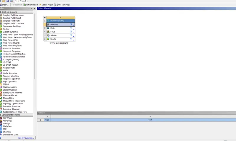
Open Ansys Fluent in workbench

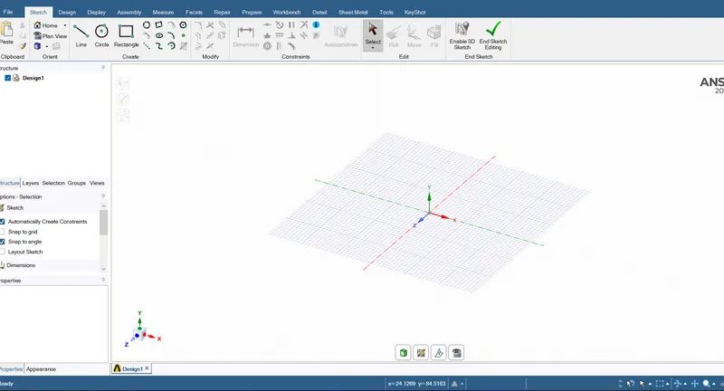
Opening spaceclaim in fluent

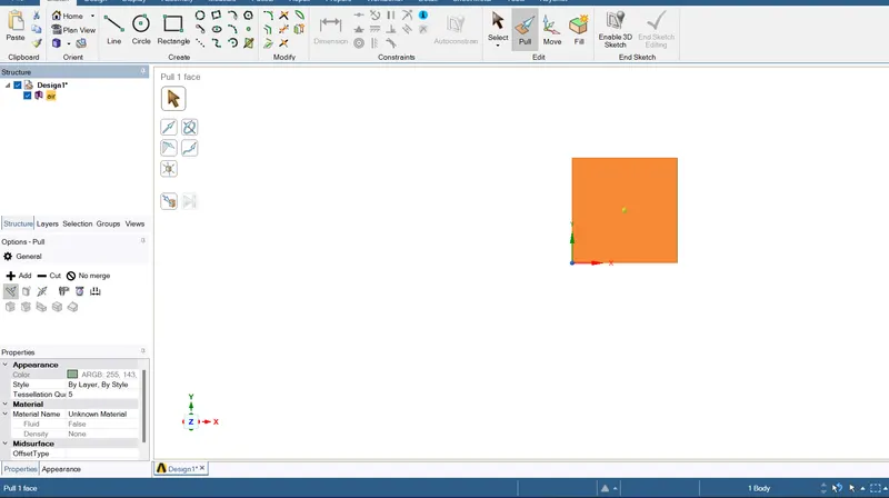
Created air surface

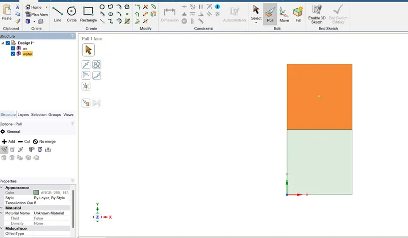
Created water surface also

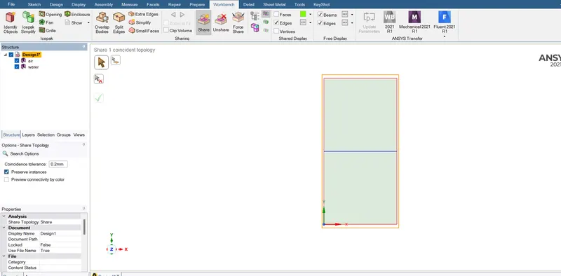
Shared topology at the interface

MESH:

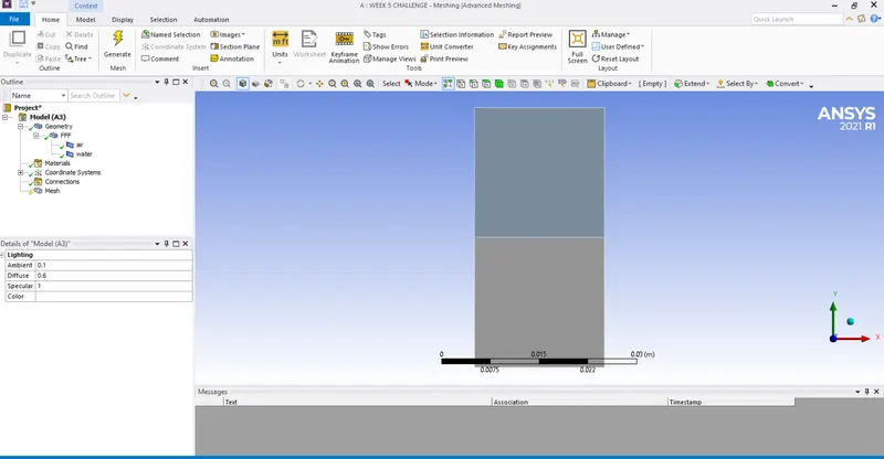
Geometry opened in Mesh window

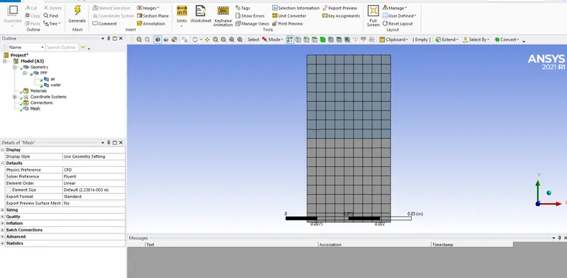
Created default mesh

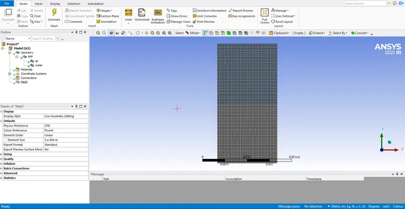
Created 0.5 mm mesh

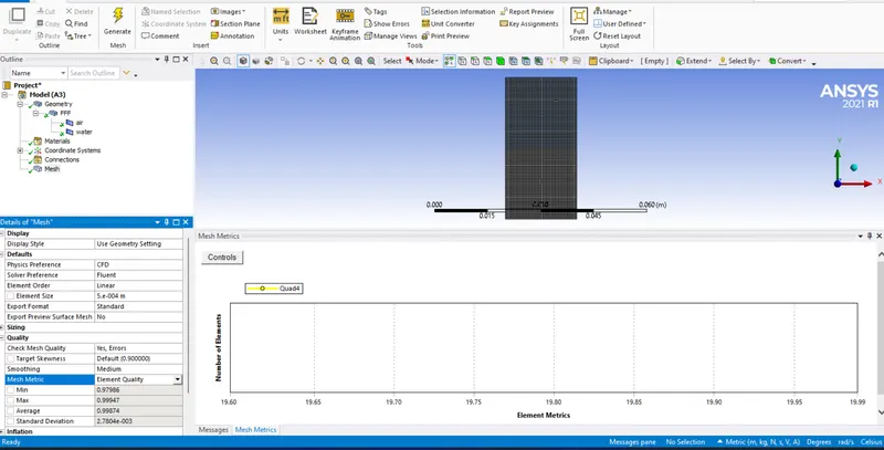
Checking quality of mesh

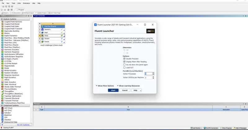
Opening setup window

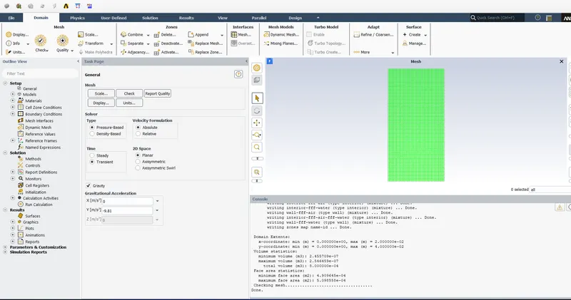
Giving value for gravity and selecting transient mode

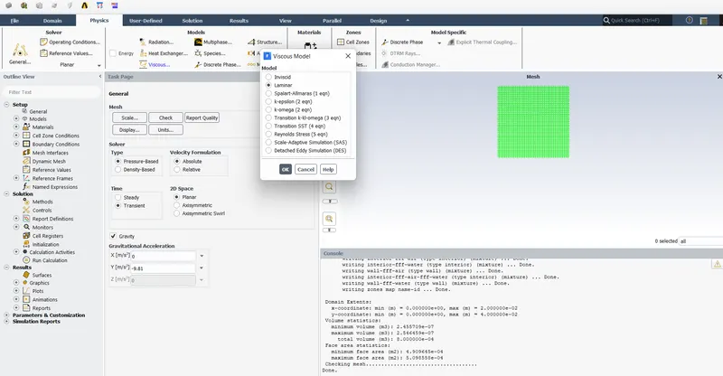
Selecting laminar flow

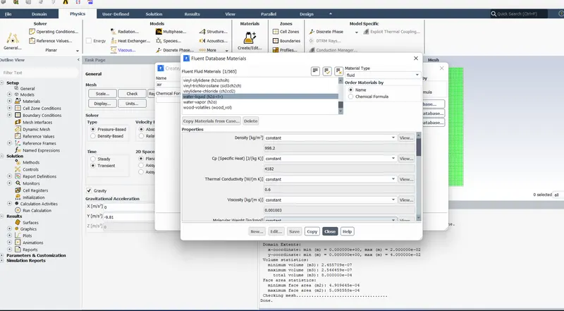
Selecting water-liquid as material from fluent database

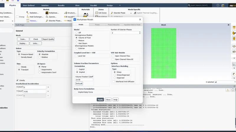
Selecting Volume of method and implicit mode

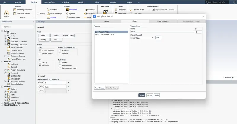
Setting primary phase as air and secondary phase as water

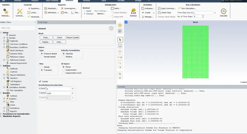
Done standard initialization

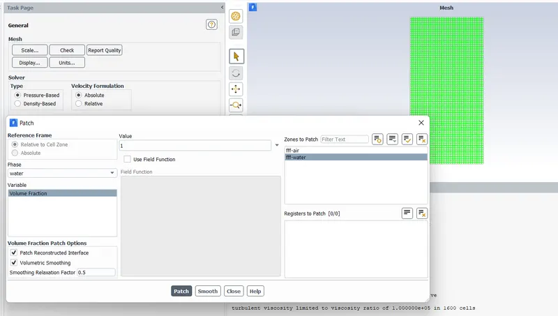
Done patching

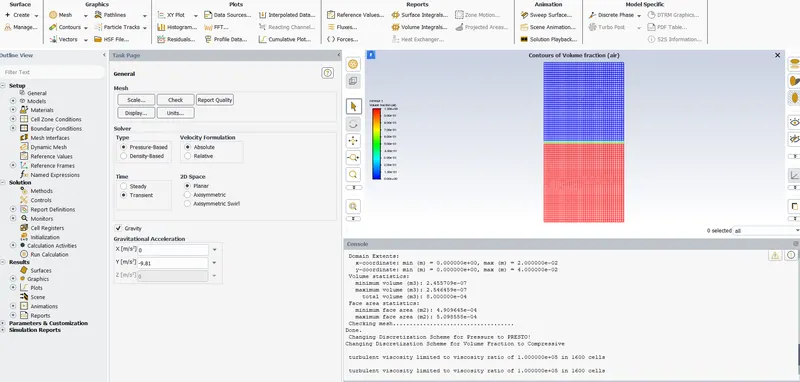
Checking whether patching done properly by creating contour

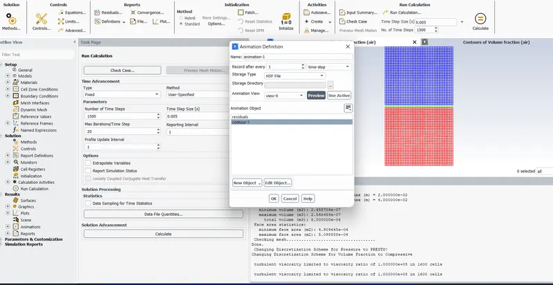
Creating animation

RESULTS AND DISCUSSION:

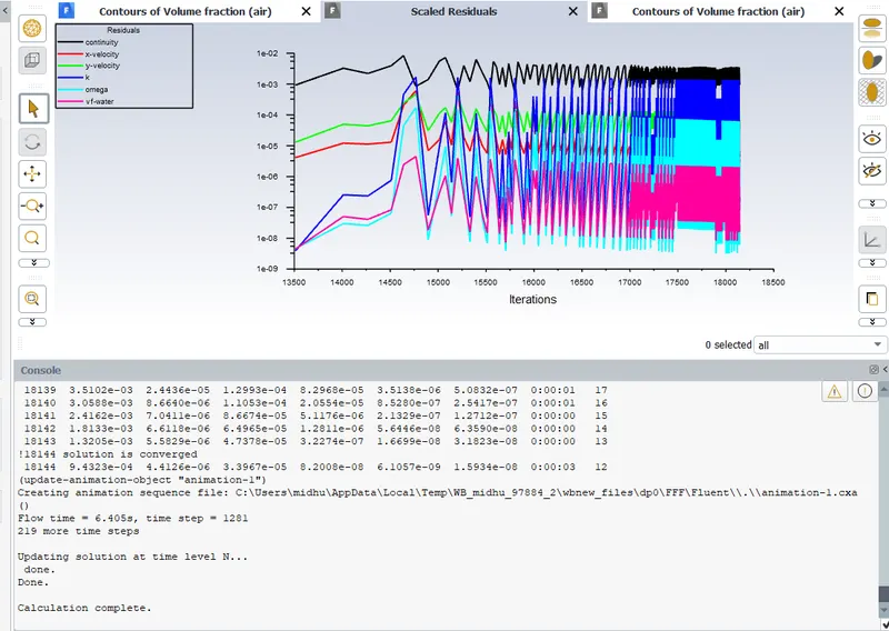
Showing residuals

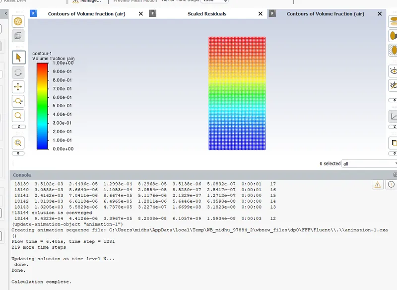
Showing contour of volume fraction for 1500 timesteps

Note: Video for this case is uploded below as "animation 1 for 0.5mm"

CASE 2:

Case 2: refined mesh with an elemental size of 0.3mm and having the fluid materials air and water.

elements=8978

timestep size=0.005

no. of timestep=1500

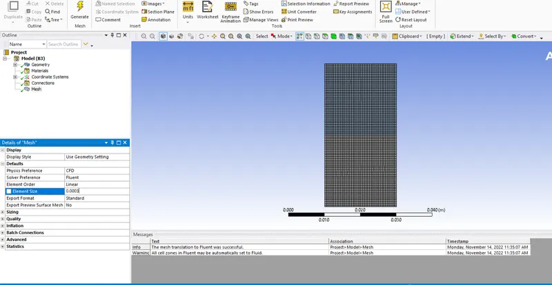
Giving mesh size as 0.3mm

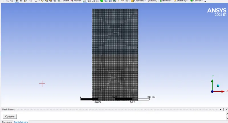
Done meshing with 0.3mm mesh

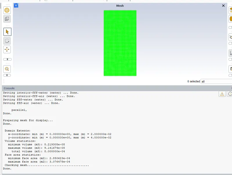
Quality of mesh checking done

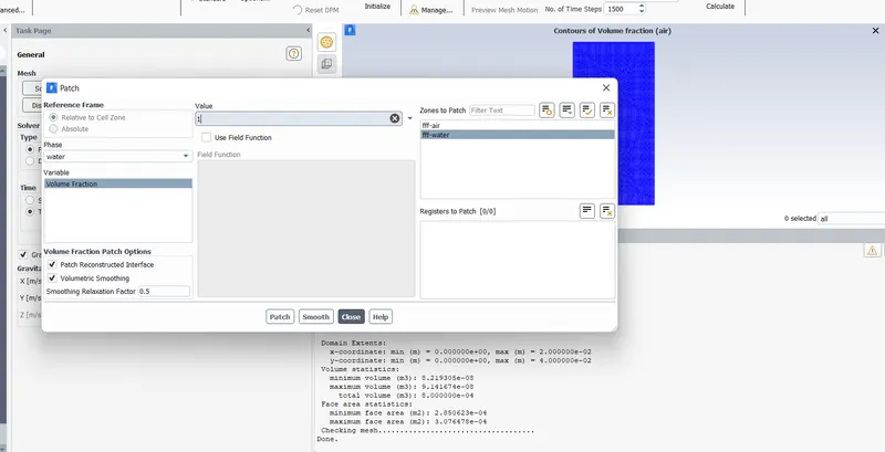
Patching done

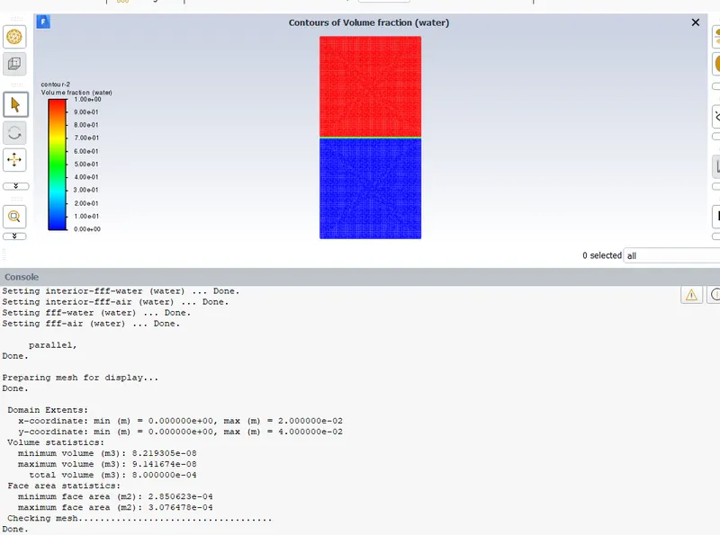
Contour of volume fraction of water indicates patching done properly

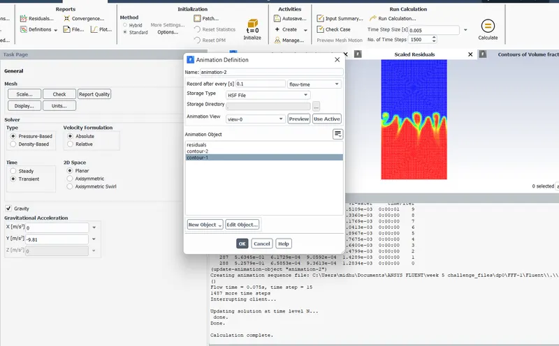
Animation created

RESULTS AND DISCUSSION:

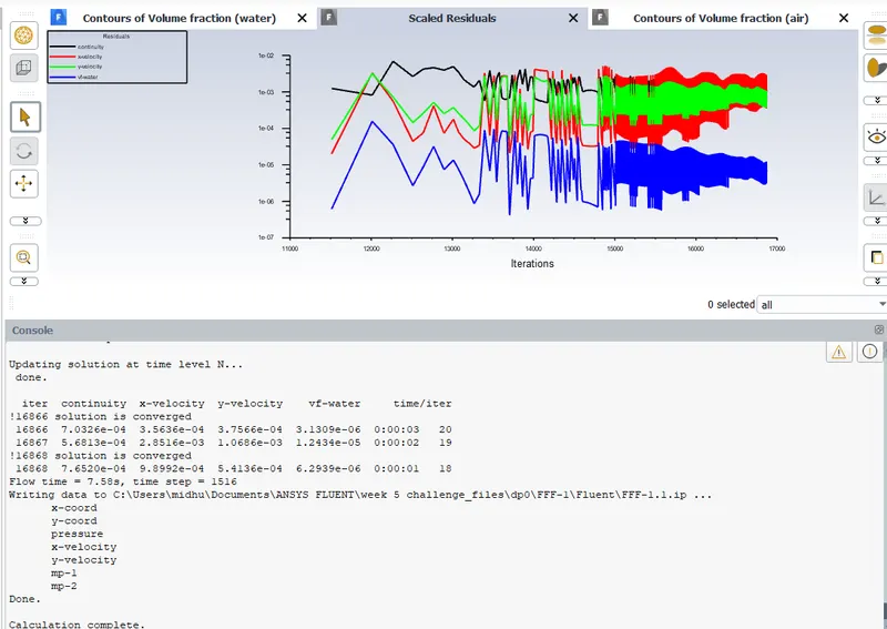
Showing residuals

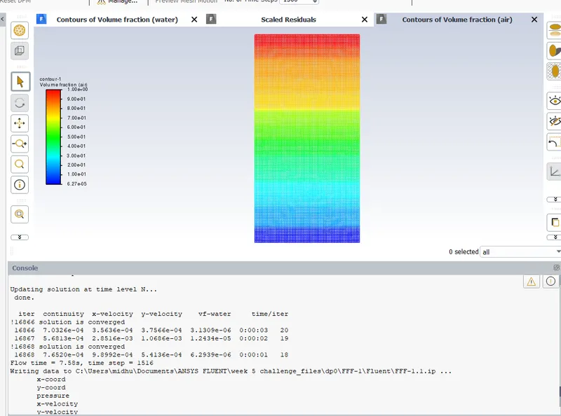
Showing contour of volume fraction of water after mixing

Note: Video for this case is uploded below as "animation 2 for 0.3mm"

Case 3: refined mesh with an elemental size of 0.3mm and having the user material(Density=400kg/m3 and viscosity=0.001kg/m-s) and water.

elements=8978

timestep size=0.005

no. of timestep=1500

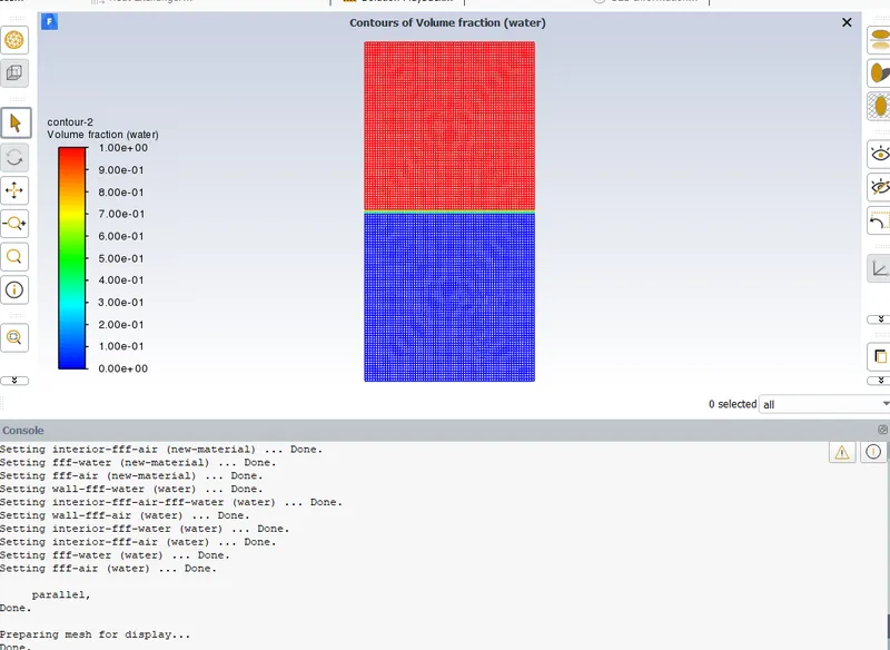
Patching done properly by checking the contours of volume fraction

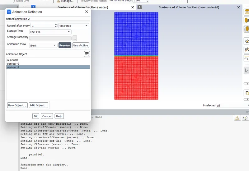
Creating animation

RESULTS AND DISCUSSION: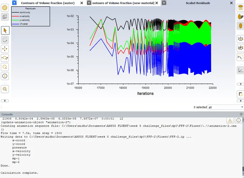

Showing residulas

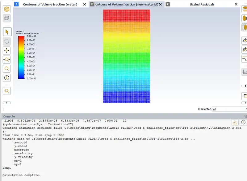
Showing contour of volume fraction of water after simulation

NOTE:Video for this case is uploded below as "animation for user defined material"

CASE 4:Simulation running with user defined material and water with explicit scheme

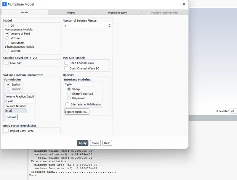
Using explicit scheme with Courant number 0.5

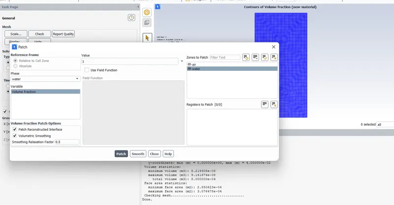
Patching done

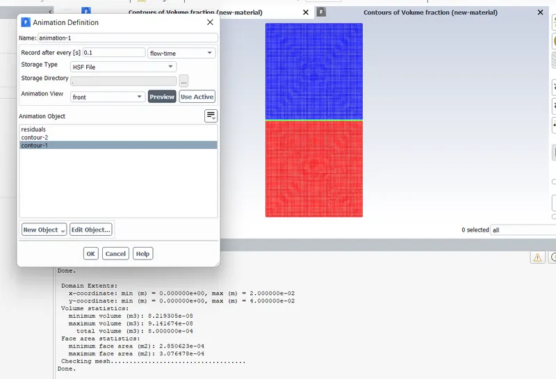
Animation created

RESULTS AND DISCUSSION:

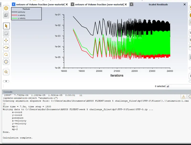
Showing residuals

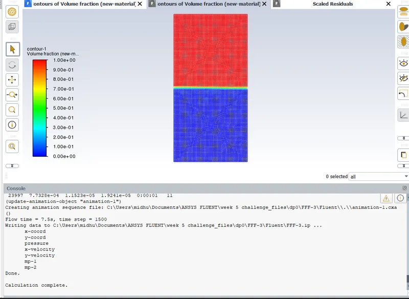
Showing contour of volume fraction of user defined material after simulation

NOTE:Video for this case is uploded below as "animation with user defined material and explicit form"

Why a steady state approach might not be suitable for these types of simulation.

• Transient solver better capture the flows.
• Transient solver can be used to run at a smaller time step, it can also run at varying time step.
• Smaller time steps are required to understand the instabilities which is only possible with transient solver.
• we expect more accuracy from transient simulation because it is time marching solution.
• Steady state simulation ignores many of the cross terms and higher order terms dealing with time.

Case 1:For fluid materials air and water

ρ1=density of water=998.2kg/m^3

ρ2=density of air=1.225kg/m^3

A=998.2−1.225/(998.2+1.225)

A=0.9975

Case 2:For fluid materials user defined and water

ρ1=density of water=998.2kg/m^3

ρ2=density of user defined=400kg/m^3

A=998.2−400/(998.2+400)

A=0.427

The difference in the fluid densities divided by their sum is defined as the Atwood number A.

For A close to 0, RT instability flows take the form of symmetric "fingers" of fluid; for A close to 1, the much lighter fluid "below" the heavier fluid takes the form of larger bubble-like plumes.

Conclusions:

In the above challenge, the simulation starts with the state of hydrostatic equilibrium, and the Rayleigh Taylor instability is observed at the interference when a lower density fluid pushes a higher density fluid due to which formation of shock waves at the interface takes place. Formation of air bubbles starts taking place, which compresses the heavy fluid around it, due to which shock waves of multidimensional fashion generates and it gets more stronger as it moves upward.

It is observed that the more we refine the mesh, the more the simulation results get smoother about the irregularities that take place at the interface of the two fluids. As higher density fluid replaces lower density fluid, the formation of air bubbles and vortex takes place, which travels towards the upward region with time.

When I used user defined material it is observed that the time for seetling down was more and this is beacuse here the difference in densities of two fluid were less.

When I used explicit form with Courant number 0.5 instead of implicit form, I observed that after simulation two fluids completly settle down and completly seperated as two regions and there was no portion of mixing region after simulation