Week 5 - Rayleigh Taylor Instability

Aim:- Perform Rayleigh Taylor Instability simulation for different mesh sizes

Tools used :-

1) Space claim

Rectangle , 3d view, share topology

2) Ansys mesh

Sizing , update, generate mesh

3) Ansys fluent

Turbulence model , Material , Multiphase , Initialization, patch , Animation , Timestep ,Calculate

4) CFD Post

Plane , Animation

Theory :-

Multiphase simulation:-

In multiphase analysis simulation , CFD is used to solve the problem the simultaneous interaction of more than one combination of phases of gases, solids or fluids.

Multiphase flows take place in a wide range of engineering applications such as power generation, water treatment, oil production, water desalination, refrigeration and air conditioning, and carbon capture and sequestration, as well as in other systems such as food and material handling processes.

Volume of Fluid (VOF)

In CFD, Volume of fluid method is a free surface modelling technique, a numerical technique for tracking anf locating the fluid-fluid interface. In VOF, , the numerical technique allows to accommodate the evolving shape of the interface.

It has application in the field of Stratified flows, sloshing, motion of large bubble in liquid, motion of liquid after dam break,prediction of jet breakup

Rayleigh Taylor Instability (RTI)

It is an instability at the interface between two fluids having different densities or different properties where low density fluid pushes high density fluid. it is the dynamic process where two fluids seeks to reduce their combined potential energy.

Like water suspended above oil in the gravity of earth , Collpase of cavitaion bubble , Mushroom clouds over volcanic eruption , atmospheric nuclear explosions.

RTI occurs in large scale also like interstellar gas, pushed out of the galactic plane by magnetic fields and cosmic rays, It plays a crucial role in fusion , Supernova.

Practical CFD models that have been based on the mathematical analysis of Rayleigh Taylor waves are :-

1) Saffman-Taylor instability

- It is also known as viscous fingering ,in this there is formation of pattrens in a morphologically unstable interface between two fluid in a porous medium. It can be seen drainage systems.

It is similar to rayleigh-taylor instability , here fluids have different viscosity and less viscous fluid is injected into high viscous fluid where in rayleigh-taylor instability there is less density fluid is pushed in more density fluid with gravity.

2) Richtmyer-Meshkov instability (RMI)

- This instability occurs in fluid flow where shock wave produced impinge upon an interface seperating two gases having different densities, this shock interaction is incompressible .

It can also be produced by the impulsive acceleration of two incompressible fluids. And by this , Richtmyer–Meshkov instability is related to Rayleigh–Taylor instability, and is often referred to as impulsive Rayleigh–Taylor instability.

3) Kelvin-Helmholtz Instability (KHI)

- KHI is a hydrodynamic instability in which immiscible, incompressible, and inviscid fluids are in relative and irrotational motion.

In KHI, the velocity and density profiles are uniform in each fluid layer, but they are discontinuous at the interface between the two fluids. This discontinuity in the velocity, i.e., the shear flow, induces vorticity at the interface; as a result, the interface becomes an unstable vortex sheet that rolls up into a spiral.

The basic mechanism of KHI is in the existence of a uniform velocity shear and that does not need gravity or density difference. KHI is treated as a fluid instability that a lighter fluid is superposed on a heavier fluid.

It is similar to RTI , onlt difference is in KHI , lighter fluid is superimposed on a heavier fluuid and no need of gravity

KHI, RTI, and RMI have different linear growth rates so they can be distinguished at linear stage but when they reach full nonlinear stage and interfacial motion with roll-up appears they can't be distinguished and treated as KHI only.

4) Plateau-Rayleigh instability

- It is aslo called Rayleigh instabilty. PRI tells the phenomena of falling stream of breaking of fluid into smaller packets with same volume but less surface area.

It is related to Rayleigh-taylor instability and is mainly used in ink jet technology and to study water dripping from Tap/Faucet ,where a jet of liquid is purturbed into a steady stream of droplets. In case of PRI, the driving force is surface tension.

Procedure;-

1) Pre-processing

Geometry

a) open space-claim

b) select a plane

c) create two surface of dimension 20mm * 20mm for two phases

d) share the topology using share option.

Meshing

a) Open the created geometry in Ansys meshing

b) create mesh with different element size

Cases	Element size	Element number
Case 1	0.5mm	3200
Case 2	0.3mm	8978
Case 3	0.1mm	80000

2) Solving

Setup

a) Open Ansys fluent

b) The simulation has to be done in transient condition so select transient state

c) Here, high density liquid is suspended with gravity so give gravity value -9.81 m2/s (negative sign due to downward diraction)

d) Select Laminar turbulence model

e) Give two material for fluid for two phases having different density which is

Cases	Material	Density	Viscosity
Case 1	Air + water	1.225 , 998.2	1.789*10^-5 , 0.001003
Case 2	Air + Water	1.225 , 998.2	1.789*10^-5 , 0.001003
Case 3	User defined material + Water	400 , 998.2	0.001 , 0.001003

f) Go to multihase option , select volume of fluid and implicit scheme

g) give phase name , first phase to be Air and secondary phase to be water for Case 1 and 2

Also for Case 3 , first phase to be user defined material and second phase to be water

h) Now do initialize and patch

i) Compute the problem with timestep size 0.01 and for 500 times so interation will be for 5 sec

3) Post Processing

a) Open CFD-Post

b) create plane and animate the simulation.

Result:-

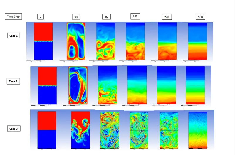
The above figure shows the simulation of Rayleigh taylor instability for 3 different cases at different time-steps, the simulation was for 0.01 time-step size and for 500 times so simulation time is 5 sec. Here transient state was employed to simulate because there is two different phase material with different density are available and are mixing, so with time properties are changing i.e., heavier fluid is coming down due to gravity and lighter fluid is going up, therefore at different time different property we can observe in the figure, hence transient state condition is used here and not steady state . If steady state condition was employed here, then change in properties cannot be observed with time.

Also three cases are there , at each cases mesh is more finer than before .In first 2 cases material is water and air whereas in case 3 material is water and user defined material whose density is less than water which is 400 kg/m3.

In first two cases , with time-step we can observe more stability and in case 3 there is less stability but there is proper mixing of contour with more clarity present. Also, in case 1 and 2 there is immediate transfer of fluid taking place whereas in case 3 at time step 162 and 228 , both materials is still mixed but in case 1& 2 it is opposite because there is not much difference in density between water and user defined material as compared to water and air.

Atwood number:-

It is dimensionless number in fluid dynamics used in hydrodynamics instabilities study. It is an important parameter to study Rayleigh-taylor instability, where penetration distance of heavier fluid into lighter fluid is given by

Agt^2

where, A = (heavier fluid density - lighter fluid density)/ (heavier fluid density + lighter fluid density)

g = acceleration due to gravity

t = time

Let A1 = Atwood number for case 1

A2 = Atwood number for case 3

D1 = Penetration distance for case 1

D2 = Penetration distance for case 3

t = time is 5 sec

Also, When Atwood number close to 0, RT instability flows take the form of symmetric “fingers” of fluid;

for Atwood number close to 1, the much lighter fluid “below” the heavier fluid takes the form of larger bubble-like plumes.

Upon calculation, A1 = 0.997 & A2 = 0.427

and D1 = 244.51 & D2 = 104.72

A1 is close to 1 and A2 is close 0 which tells that in case 1, RT instability flows takes the form of symmetric of fluid and in case 2,RT instability flows takes the form of bubble like plumes which can be seen in above figure.

Google drive link for animation :-

https://drive.google.com/drive/folders/1vrPooCeWm6Qw3oOXF-V6lOy-kW2bWT8v?usp=sharing