Week 5 - Rayleigh Taylor Instability

AIM:

  In this challenge the analysis of the  Rayleigh Taylor instability simulation is must be carried out along with the answers of the follwing questions:

1. What are some practical CFD models that have been based on the mathematical analysis of Rayleigh Taylor waves? In your own words, explain how these mathematical models have been adapted for CFD calculations.
2. Perform the Rayleigh Taylor instability simulation for 2 different mesh sizes with the base mesh being 0.5 mm. Compare the results by showing the animations( Attach them from your google drive). Observe the differences in the animation and explain the effect of mesh size on simulation. Also, explain why a steady-state approach might not be suitable for these types of simulation.[ Choose Air and Water for this simulation]
3. Run one more simulation with water and user-defined material(density = 400 kg/m³, viscosity = 0.001 kg/m-s) for refined mesh. 
4. Define the Atwood Number. Find out the Atwood number for both the cases and explain how the variation in Atwood number in the above two cases affects the behavior of the instability. 

the answers for this questions is also should be attached in the report.

The Rayleigh–Taylor instability, or RT instability is an instability of an interface between two fluids of different  densities  which occurs when the lighter fluid is pushing the heavier fluid.

INTRODUCTION:

The rayleigh taylor instability will be analysis in the ansys workbench with the help of the fluid flow (fluent).
The fluid flow simulations contains several steps are :
1.geometry
2.Meshing
3.Setup
4.Solution
5.Results.
By the help of all this software the rayleigh taylor instability is analysied properly and completely.

GEOMETRY:

The space claim is opened and in the sketch mode in the XY-plane the square is create dwith the dimensions of 20*20 mm.
Click on the pull tool and click the surface of that square and make that into 2D body.
Right click on the design in the toolbar and create bthe new component and name it as air.

Then create the another new component and name it as water.
After create the water,new sketch is enabled and a squareis created above the already existed one.
the dimensions of the new square is also 20*20 mm.

Finally in the workbench deck of the space claim use share prep and click on the two square and click ok.
Now the 2 edges are share their edges at that intermediate pointof the 2 surfaces.

MESHING:

The space claim 2D is updated in the ansys workbench and the mesh is opened.
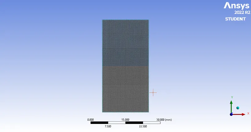
After the model is loaded in the mesh interface ,the element size is changed to 0.5 mm.

In order to get the fine and depth analysis of the instability between the two layers of the surfaces(air,water.)

The refined mesh of the surfaces is shown below:

SETUP:

The update of the project in the ansys workbench is carried out after finishing the mesh .
Now the setup is opened,the model is loaded completely in the ansys fluent.
The domain settings are changed into the transient time because the analysis collapse of the 2 surfaces will be carried.

Gravity is also enabled and the Y-axis value is changed as -9.81 m/s.
Then in the setup physics deck the multiphase is opened and the method is changed as volume of fluid and put the implicit method.

Now the materials is opened materials - fluent database-clcik on h2o-l(water liquid) and copy.
now the materials is available of both water and air.

Then the phases section is opened which is present in the multiphases,change the phase 1 into air and phase2 into water and click ok.

In solving deck,click on intialize with the standard intilaize.no changes occur in the console.
Click on patch and change the phase as water and click volume fraction in variable.
Mention the value as 1 for water and patch. change the value as 0 for air and patch and close.

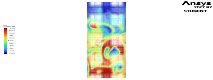
Now go the resuls deck ,open the new contours and create the volume fraction contour in the phases,select water in phases.
click every part of the surfaces and clcik save/display.


Now come back to the solution deck in the animation tool bar use solution animations and create the contour-1 .
Finally in the calculation set up the step size is 0.005 and number of time steps is 1500.and calculate.

CASE1(MESH LENGTH=0.5MM):

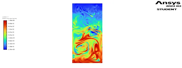
the  velocity contour of the collapse in the tow surfaces (air and water) diagram is shown below:

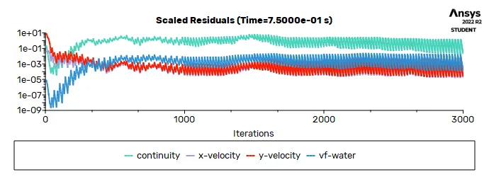
the residual  of the collapse in the 2 surfaces (air and water) diagram is shown below:

 CASE2 (MESH LENGTH=0.4MM):

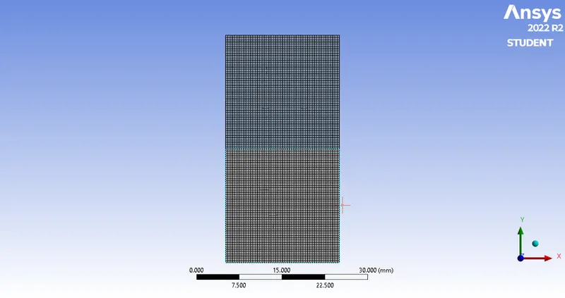
the mesh is refined ,the mesh length is 0.4 mm .

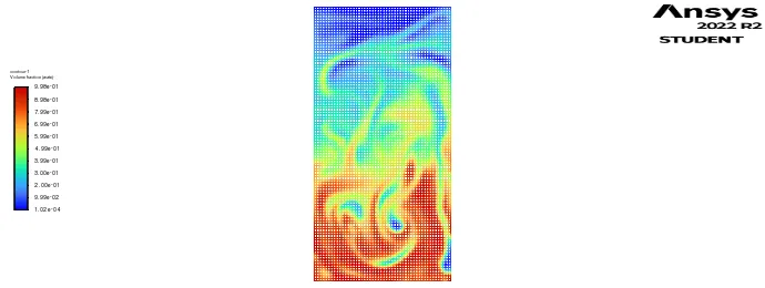
then do the same setup procedure and the resuidual and velocity contour is.

The refined mesh of the surfaces is shown below:

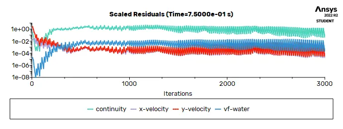
the residual  of the collapse in the 2 surfaces (air and water) diagram is shown below:

the  velocity contour of the collapse in the tow surfaces (air and water) diagram is shown below:

CASE 3 (MESH LENGTH=0.2MM):

the mesh is still refined , the mesh length is 0.2 mm.

In the setup also density = 400 kg/m³, viscosity = 0.001 kg/m-s is changed  for this  refined mesh.

then the same procedure for the setup is chaged and the calculation is carried out.

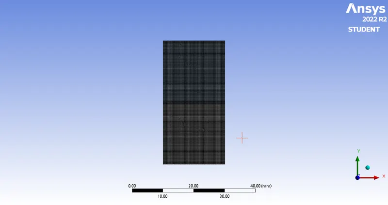
 The refined mesh of the surfaces is shown below:

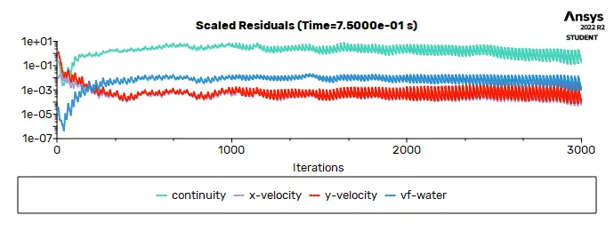
the residual  of the collapse in the 2 surfaces (air and water) diagram is shown below:

the  velocity contour of the collapse in the tow surfaces (air and water) diagram is shown below:

ATWOOD NUMBER:

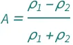
The Atwood number is a dimensionless number in fluid dynamics used in the study of hydrodynamic instabilities in density-stratified flows.