Week 5 - Rayleigh Taylor Instability

Challenge 5

Aim: -

CFD simulation of Rayleigh Taylor Instability of air and water for different mesh parameters and user material and water for different mesh length

Objective: -

1. What are some practical CFD models that have been based on the mathematical analysis of Rayleigh Taylor waves? In your own words, explain how these mathematical models have been adapted for CFD calculations.
2. Perform the Rayleigh Taylor instability simulation for 2 different mesh sizes with the base mesh being 0.5 mm. Compare the results by showing the animations (Attach them from your google drive). Observe the differences in the animation and explain the effect of mesh size on simulation. Also, explain why a steady-state approach might not be suitable for these types of simulation. [ Choose Air and Water for this simulation]
3. Run one more simulation with water and user-defined material (density = 400 kg/m³, viscosity = 0.001 kg/m-s) for refined mesh.
4. Define the Atwood Number. Find out the Atwood number for both the cases and explain how the variation in Atwood number in the above two cases affects the behaviour of the instability.

Introduction: -

Fluid instability

Fluid instabilities occur in a stratified fluid system when the light fluid is accelerated into the heavier one often by means of a pressure gradient.

Different types of instability

1. Rayleigh–Taylor instabilityof an interface between two fluids of different densities which occurs when the lighter fluid is pushing the heavier fluid.

As the RT instability develops, the initial perturbations progress from a linear growth phase into a non-linear growth phase, eventually developing "plumes" flowing upwards (in the gravitational buoyancy sense) and "spikes" falling downwards. In the linear phase, the fluid movement can be closely approximated by linear equations, and the amplitude of perturbations is growing exponentially with time. In the non-linear phase, perturbation amplitude is too large for a linear approximation, and non-linear equations are required to describe fluid motions. In general, the density disparity between the fluids determines the structure of the subsequent non-linear RT instability flows (assuming other variables such as surface tension and viscosity are negligible here). The difference in the fluid densities divided by their sum is defined as the Atwood number, A. For A close to 0, RT instability flows take the form of symmetric "fingers" of fluid; for A close to 1, the much lighter fluid "below" the heavier fluid takes the form of larger bubble-like plumes.

Ex : water and air mixing, supernovae

2. Saffman–Taylor instability

   formation of patterns in a morphologically unstable interface between two fluidsin a porous medium

3. Kelvin–Helmholtz instability occurs when there is velocity shearing a single continuous fluid or a velocity difference across the interface between two fluids.
4. Richtmyer–Meshkov instability occurs when two fluids of different density are impulsively accelerated.
5. Plateau–Rayleigh instability falling stream of fluid breaks up into smaller packets with the same volume but less surface area.

Application: -

supersonic aviation (ramjet engines) and high-energy-density processes like inertial confinement fusion (ICF), which is key to achieving energy from fusion.

Solving & Modelling approach

Geometry setup

It’s a 2d model so it can sketch in spaceclaim application for that need to draw 20mm 2 box and surface formed using pull command and name below solid as air and above as water and move both to single component and to share information from one box to another share topology is enabled in workbench section once one with above process close the application

Mesh

Just need to change the element size in mesh according to reequipment

And name the below part as air and above one as water and mesh it and close the application

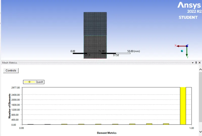
fig 1 element quality for 0.5mm mesh length

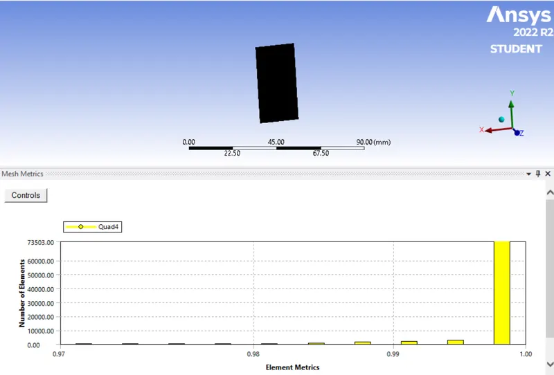
fig 2 element quality for 0.1 mm mesh length

Setup

• In setup solver section select type as pressure based, velocity formulation as absolute and time as transient
• Select gravity and give gravity in y direction as -9.81 m/s^2
• Viscous model as laminar model
• In multi-phase model select volume of fluid and implicit formulation
• In material air and water is selected
• In solution section initialization as standard and initialize then patch
• Contour is created of phase change and animation is created using contour
• Calculate the solution for required no of time step
• Calculation is doe using animation frame animation video is created
• Same step followed to simulate with user material just changing the material

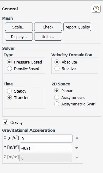
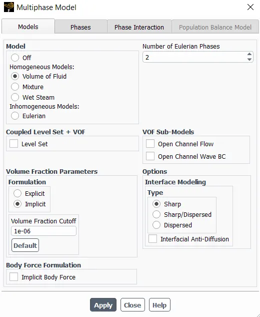
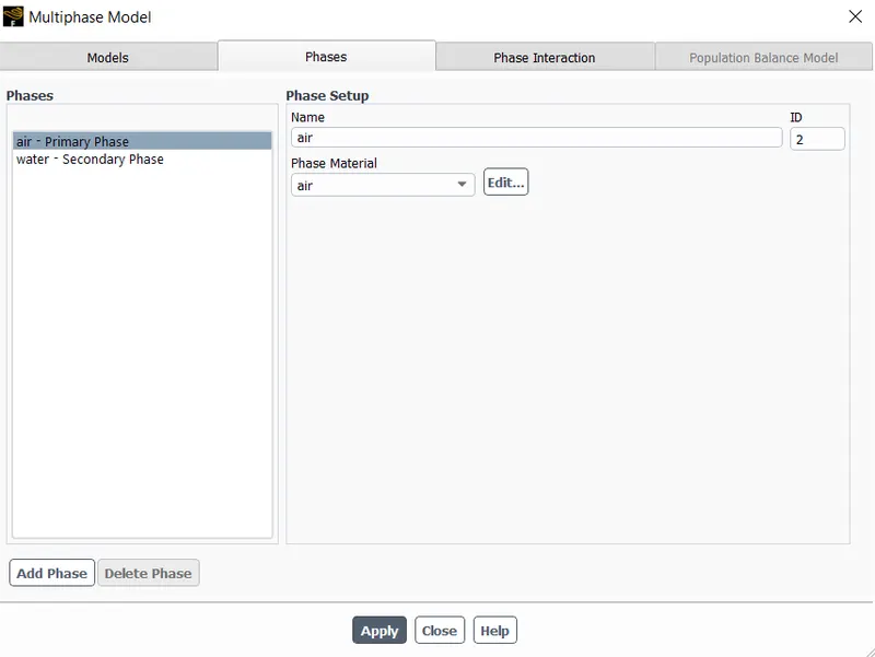
fig 3 setup for simlation

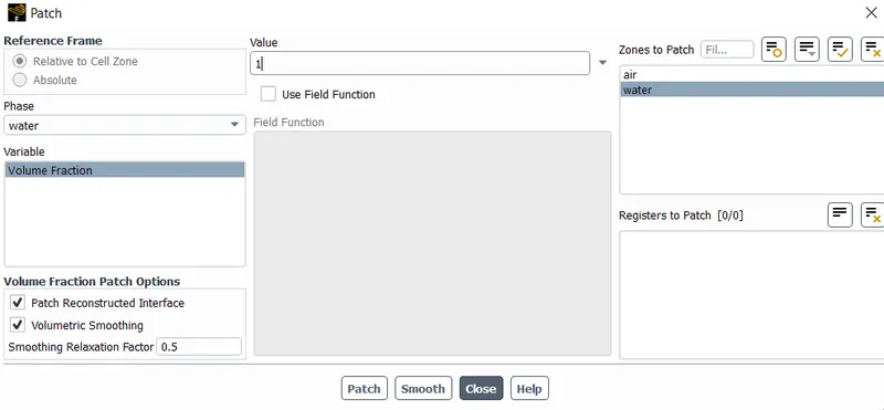
fig 4 patch parameter

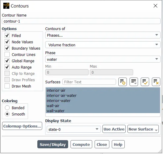
fig 5 contou parameter

Atwood number

is a dimensionless number in fluid dynamics used in the study of hydrodynamic instabilities in density stratified flows.

`A=(rho_1-rho_2)/(rho_1+rho_2)`

case 1 air and water

`A=(998.2-1.225)/(998.2+1.225)`

A=0.9975

case 2 usermaterial and water

`A=(rho_1-rho_2)/(rho_1+rho_2)`

`A=(998.2-400)/(998.2+400)`

A=0.4278

atwood number waries from 0 t 1 o bing same density fluid and 1 being the heaver fluid then other

Conclusion

If fluid is relatively higher denser then the other fluid less bubble formation takes place

As the mesh becomes fine the animation or the solution looks cleaner and more authentic