Challenge

Week 5 - Rayleigh Taylor Instability

HHerbert Rathna Singh G2 Sept 2022

CFD

Aim: To analyse the Rayleigh Taylor waves.

Objective:

To Perform the Rayleigh Taylor instability simulation for air and water with 2 different mesh sizes with mesh size 0.5 mm and 0.1mm and compare the results by showing the animations. We will observe the differences in the animation and explain the effect of mesh size on simulation and also, explain why a steady-state approach might not be suitable for simulation types of simulation.
To simulate with water and user-defined material(density = 400 kg/m³, viscosity = 0.001 kg/m-s) for refined mesh.
To define the Atwood Number and find out the Atwood number for both the cases and explain how the variation in the Atwood number in the above two cases affects the behaviour of the instability

SOLUTION:

Rayleigh–Taylor instability :

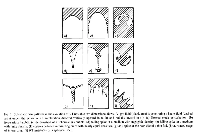
The Rayleigh–Taylor instability or RT instability is the instability of an interface between two fluids of different densities which occurs when the lighter fluid is pushing the heavier fluid.
Examples include how water behaves when it is suspended above oil in the gravitational field of Earth, mushroom clouds caused by volcanic eruptions and nuclear explosions in the atmosphere, supernova explosions in which the expanding core gas is accelerated into the denser shell gas, instability in plasma fusion reactors, and inertial confinement fusion.
A common example of Rayleigh-Taylor instability is the suspension of water over oil. This instability can be modelled by two layers of immiscible fluid that are completely parallel to one another, with the denser fluid sitting on top of the less dense one and both being subject to gravity.

Saffman–Taylor instability :

When a more viscous fluid is displaced by a less viscous fluid, the interface becomes unstable. However, when the opposite occurs and one viscous fluid is displaced by the other, no instability is evident. If the interface is horizontal and separates two fluids of different densities, with the heavier fluid being above the lighter one, essentially the same effect occurs driven by gravity (without injection) and is known as the Rayleigh-Taylor instability. In the radial configuration, the pattern develops into fingers by tip-splitting repeatedly, whereas, in the rectangular configuration, the system evolves until a single finger (the Saffman-Taylor finger) forms.
Hele-Shaw cells, which are made up of two parallel glass sheets that are spaced closely apart and contain a viscous fluid, have been the subject of the majority of experimental studies on viscous fingering. The two most common set-ups are the channel configuration, in which the less viscous fluid is injected at one end of the channel, and the radial configuration, in which the less viscous fluid is injected at the centre of the cell. Additionally, biological systems are capable of self-generating instability patterns similar to viscous fingering.

Richtmyer–Meshkov instability (RMI) :

When two fluids with different densities are accelerated abruptly, the Richtmyer-Meshkov instability (RMI) develops. Usually, a shock wave will pass through to accomplish this. Small amplitude perturbations that initially increase linearly with time are the beginning stages of the instability's development. After that, a nonlinear regime sets in, where bubbles appear when a light fluid penetrates a heavy fluid and spikes appear when a heavy fluid penetrates a light fluid. The two fluids eventually combine as a chaotic regime. This instability can be thought of as the Rayleigh-Taylor instability's impulsive-acceleration limit.

Plateau–Rayleigh instability :

The Plateau–Rayleigh instability, often just called the Rayleigh instability, explains why and how a falling stream of fluid breaks up into smaller packets with the same volume but less surface area.
It belongs to a larger area of fluid dynamics that deals with fluid thread breakup and is related to the Rayleigh-Taylor instability. A specific kind of inkjet technology uses this fluid instability to its advantage by perturbing the liquid jet into a steady stream of droplets.
The Plateau-Rayleigh instability is caused by the tendency of liquids to minimise their surface area due to their surface tensions. The final pinching profile has recently undergone a significant amount of work by being attacked with self-similar solutions.

SIMULATION:

Geometry setup:

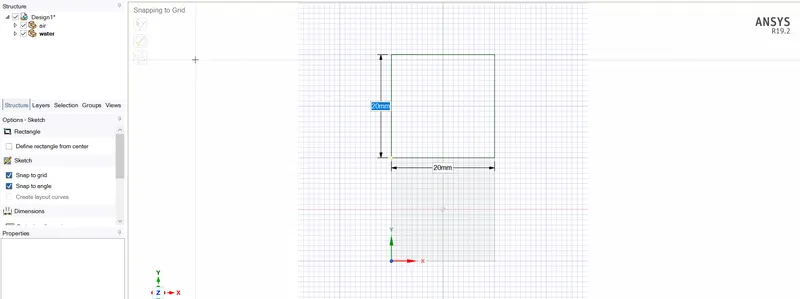
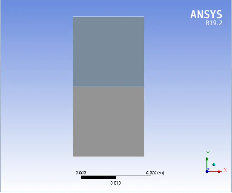
Draw a square of 20mm and use the pull tool to name it 'air'. Now draw another square of the same dimension and use the pull tool to name 'water'.
Now select both the squares and select share for conformal mesh for 'Share topology'. Check whether the surfaces are shared in the 'Share topology' option.
Make this geometry in 2D in an X-Y plane.
The geometry was created in spaceclaim and it involves no other importing of CAD models. The surface model was further processed for meshing .This preprocessing phase of the workflow is extremely important because it determines the simulation potential and limits the CFD results.
This completes the creation of geometry.Then we close the spaceClaim ,the progress will be saved automatically.

Meshing :

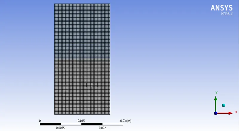
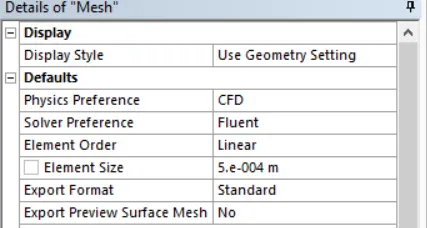
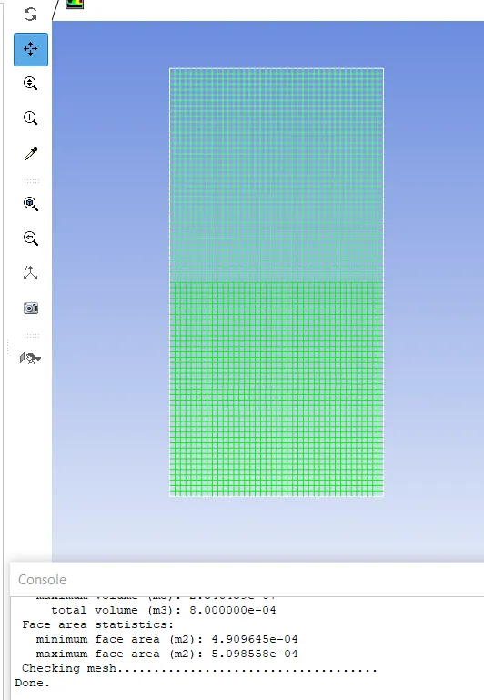
Change the mesh size to 0.5 mm from the default size.
Here our minimum quality is around 15 %,so we can move further for our solution setup.

Element size:

Setup:

CASE - 1: Rayleigh–Taylor instability between air and water with coarse mesh of size 0.5 mm :

Multiphase:

Homogeneous model: Volume of fluid

Formulation: Implicit

Primary phase: air

Secondary phase: water

We need to enable gravity by giving value for Y as -9.8 m/s^2 as gravity is acting in negative Y-direction.
Initlizing all the input setup like material selection using laminar flow, creating counter and solution animations.

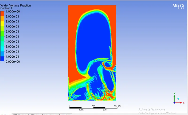
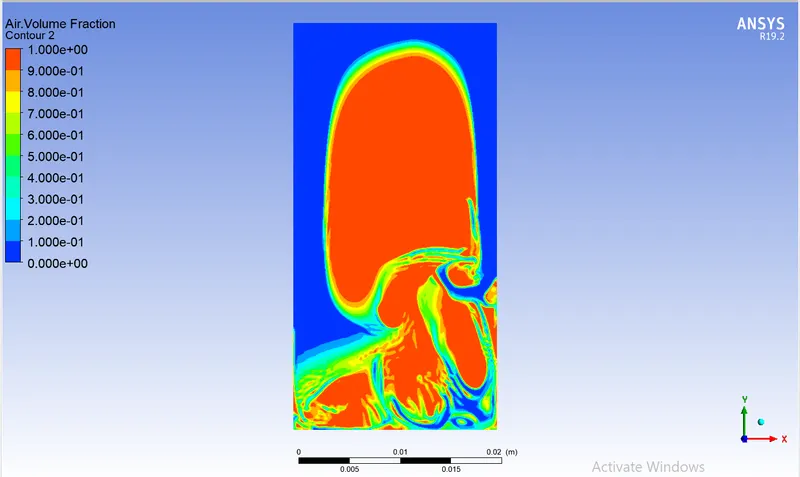
CASE -2: Rayleigh–Taylor instability between air and water with fine mesh of size 0.1 mm

Everything is same from the point of geometry and when it comes to mesh the only change is the mesh size,here it is quite refined with mesh size of 0.1 mm.
Comming to set up even it is also same.
Here we run for 1400 times steps with time step size = 0.005 and the total run time = 7s.

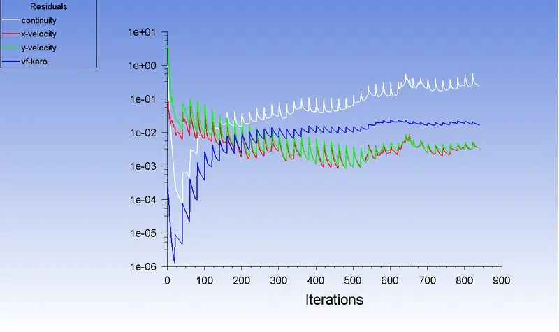
CASE- 3 :Rayleigh–Taylor instability between user defined material and water with fine mesh of size 0.1 mm :

Everything is same from the point of geometry and even when it comes to mesh, the mesh size is also same as refine case above i.e., 0.1 mm.
Comming to setup the change comes here ,we change the lighter material i.e.,from air to user defined material with density = 400 kg/m³, viscosity = 0.001 kg/m-s .
Then again every thing is same ,we patch the lighter fluid down and denser fluid upper side of the box or domain.
Then we run for 1800 times steps with time step size = 0.005 and the total run time = 9.00s.
So let us directly run the simulation then postprocess the results and compare the results with above case -2 with respect to Atwood number .

RESULTS:

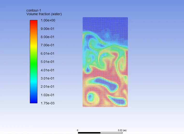
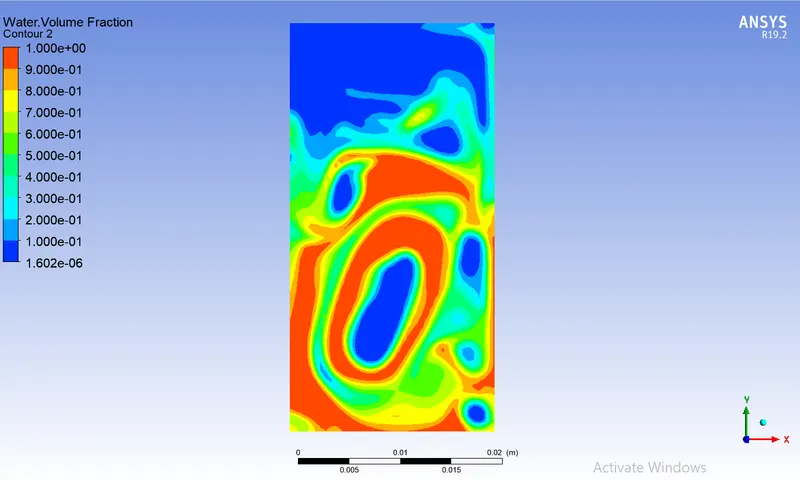
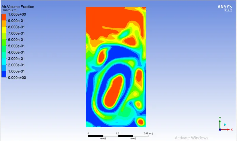
CASE - 1: Rayleigh–Taylor instability between air and water with coarse mesh of size 0.5 mm :

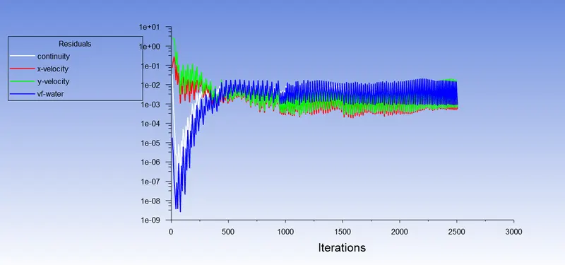
Residuals plot :

Volume fraction of water contour :

WATER Volume fraction of water contour :

AIR fraction of water contour :

Animation of Rayleigh:

https://drive.google.com/file/d/1UC_1Ra9NDMnot5FWNDZYv4UcyxpUKCw8/view?usp=sharing

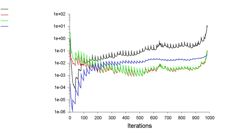
CASE -2: Rayleigh–Taylor instability between air and water with fine mesh of size 0.1 mm

Residuals plot :

Volume fraction of water contour :

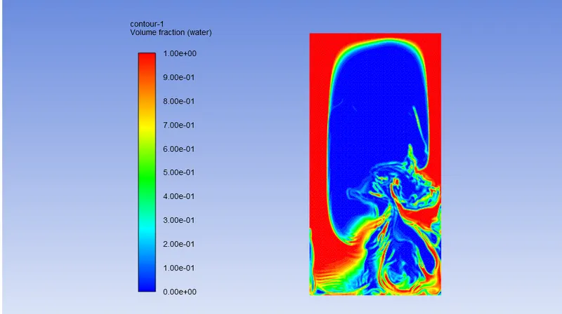
WATER Volume fraction of water contour :

AIR fraction of water contour :

Animation of Rayleigh:

https://drive.google.com/file/d/1uhcsUaeKBJMwiusc_nxZEWehVYT4Poeb/view?usp=sharing

CASE- 3 :Rayleigh–Taylor instability between user defined material and water with fine mesh of size 0.1 mm :

Residuals plot :

Volume fraction of water contour :

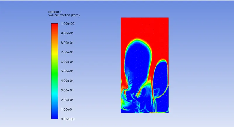
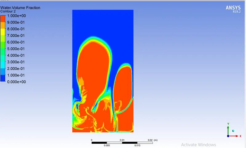
WATER Volume fraction of water contour :

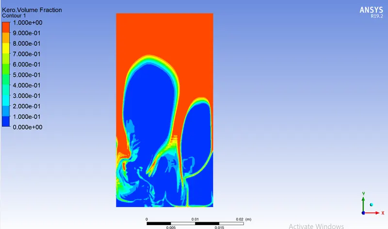
USER DEFINEND fraction of water contour :

Animation of Rayleigh:

https://drive.google.com/file/d/1V0En17Dii5kE6aElmfKh0rkmNBRe05Qq/view?usp=sharing

Atwood Number:

The Atwood number is a dimensionless number in fluid dynamics used in the study of hydrodynamic instabilities in density-stratified flows. The Atwood number equals the ratio of the difference in mass densities to their sum.

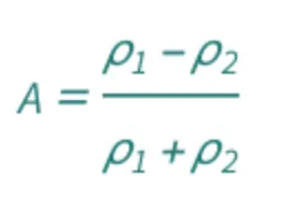
WHERE,

symbol	description	physical quantity
A	Atwood number	"AtwoodNumber"
ρ₁	fluid density	"MassDensity"
ρ₂	fluid density of lighter fluid	"MassDensity"

Case 1:

ρ1 = 1.225 kg/m^3

ρ2 = 998.2 kg/m^3

A = 0.9975

Case 2:

ρ1 = 400 kg/m^3

ρ2 = 998.2 kg/m^3

A = 0.4278

Therefore, the acceleration will be greater and the initial instability will be greater if the difference in fluid densities is greater. Later, it will do so more quickly and reach the equilibrium stage.
Therefore, it will take less time to calm down. In this instance, turbulence will increase the splashing effect. It will result in a non-linear growth rate and a more asymmetrical pattern.
On the other hand, if there is less of a disparity between the densities, there will be less acceleration and instability. The phase will gradually change. It will take longer to calm down.
In the case of a turbulence model, the splashing effect will be less noticeable, and we can symmetrical pattern and accelerating leading to linear growth rate.

CONCLUSION:

Hence, we have obtained practical CFD models that are based on the mathematical analysis of Rayleigh Taylor.
The variation in Atwood Number, where we obtained the same observation, was used to validate this numerical simulation using the observations obtained by previous researchers.
Spikes and globules were still present at the end of the simulation at lower Atwood numbers, but not at the Atwood number of 0.99 in Case 2. We also noticed that the interface thickness decreases as the mesh is refined based on the grid dependency. For In terms of computational time, transient simulation requires more than steady state simulation.
With a time step size of 0.005, the transient solver can be used to run at smaller time steps and better capture the flow. The instabilities must be observed at shorter time scales, which is only possible through transient simulation. .
Since it is a time marching solution, transient simulation is the best method for running the Rayleigh Taylor Instability calculation because it provides greater accuracy.

REFERENCE:

Week 5 - Rayleigh Taylor Instability

Ship work like this
in your own course.

Talk to a career counsellor

Ship work like thisin your own course.

Talk to a career counsellor

Ship work like this
in your own course.