Week 5 - Rayleigh Taylor Instability
Rayleigh Taylor Instability
Aim:
- To study the concept of Rayleigh Taylor Instability and some practical CFD models that have been based on the mathematical analysis of Rayleigh Taylor waves.
- To study the Rayleigh Taylor Instability simulation for 2 different mesh sizes in addition to baseline and compare the results.
- To study the effect of Atwood number variation on Rayleigh Taylor Instability for all the cases.
Given:
- Baseline mesh size= 0.5mm
- Materials selection - Air, water and user-defined material(density = 400 kg/m3, viscosity = 0.001 kg/m-s)
INTRODUCTION:
RAYLEIGH TAYLOR INSTABILITY:
The Rayleigh–Taylor instability or RT instability is the instability of an interface between two fluids of different densities which occurs when the lighter fluid is pushing the heavier fluid. Examples include the behavior of water suspended above oil in the gravity of earth, mushroom clouds like those from volcanic eruptions and atmospheric nuclear explosions, supernova explosions in which expanding core gas is accelerated into denser shell gas, instabilities in plasma fusion reactors, and inertial confinement fusion.
PRACTICAL CFD MODELS BASED ON RAYLEIGH TAYLOR WAVE:
RICHTMYER-MESHKOV INSTABILITY:
- This instability occurs when two fluids with different densities are accelerated impulsively
- Magnetized target fusion and the formation of material in the cores of stars (cobalt 56) are examples of this type of instability
VICIOUS VORTEX SINGLE-MODE BUBBLE EVOLUTION MODEL:
- Explains the viscous effect of early stages of Rayleigh Taylor wave for low Atwood number.
SAVART-PLATEAU-RAYLEIGH INSTABILITY OF A WATER COLUMN:
- A column of liquid spontaneously breaks up into droplets under the influence of the Atwood number.
K-L TURBULENCE MODEL FOR THE SELF-SIMILAR GROWTH OF THE RAYLEIGH-TAYLOR AND RICHTMYER-MESHKOV INSTABILITIES:
- Used to simulate turbulence model or turbulent boundary conditions.
VOLUME OF FLUID METHOD:
In computational fluid dynamics, the volume of fluid (VOF) method is a free-surface modeling technique, i.e. a numerical technique for tracking and locating the free surface (or fluid-fluid interface). It belongs to the class of Eulerian methods which are characterized by a mesh that is either stationary or is moving in a certain prescribed manner to accommodate the evolving shape of the interface. As such, VOF is an advection scheme—a numerical recipe that allows the programmer to track the shape and position of the interface, but it is not a standalone flow-solving algorithm.
CASE SETUP:
GEOMETRY:
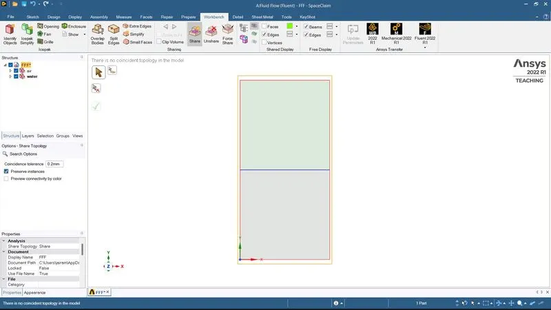
- Create a square of 20mm*20mm. Use the Pull tool in order to create a surface.
- Move the generated component to the New Component. Name it Air. Now click on design and create a new component --> Water. Repeat sketch just above the Air with similar dimensions as mentioned.
- Check if both the components i.e Air and Water are created.
- Workbench > click on Share > Ok
Mesh
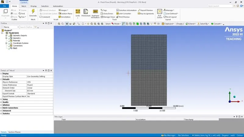
- OPEN MESH --> Generate the mesh --> baseline mesh element size (0.5mm).
SETUP:
|
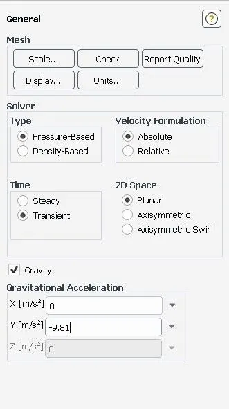
Solver Type |
Pressure-Based |
|
Velocity Formulation |
Absolute |
|
Time |
Transient |
|
Models |
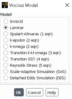
Viscous model: laminar |
|
Multiphase |
Volume of fluid : Implicit formulation : 2 phases |
|
Material |
Fluid type: Air Fluid type: water |
|
Cell zones |
Fluid type: Air : water |
|
Boundaries |
Standard |
|
Reference values |
Standard |
|
Initialization |
Standard Patch: Water-surface (1 value of volume fraction of water) : Air-surface(0 value of volume fraction of water) |
GENERAL:
Viscous MODEL:
MATERIAL:
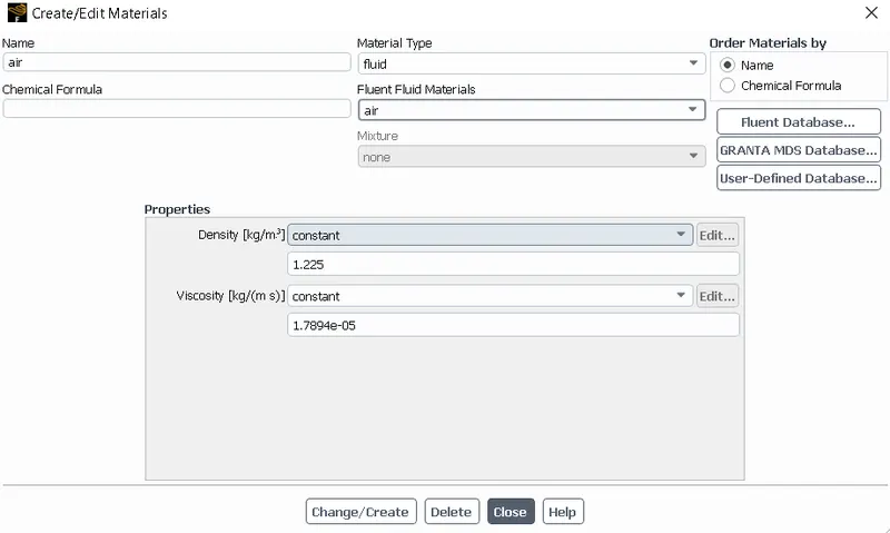
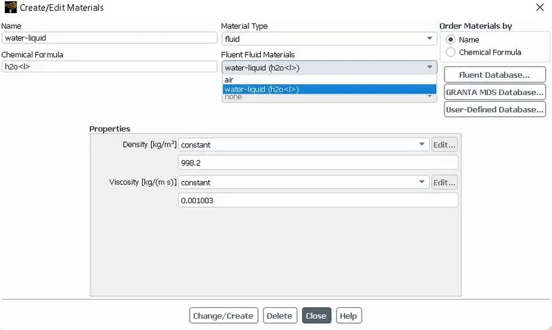
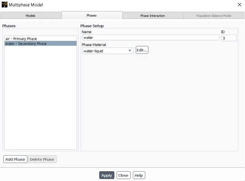
MULTIPHASE MODEL:
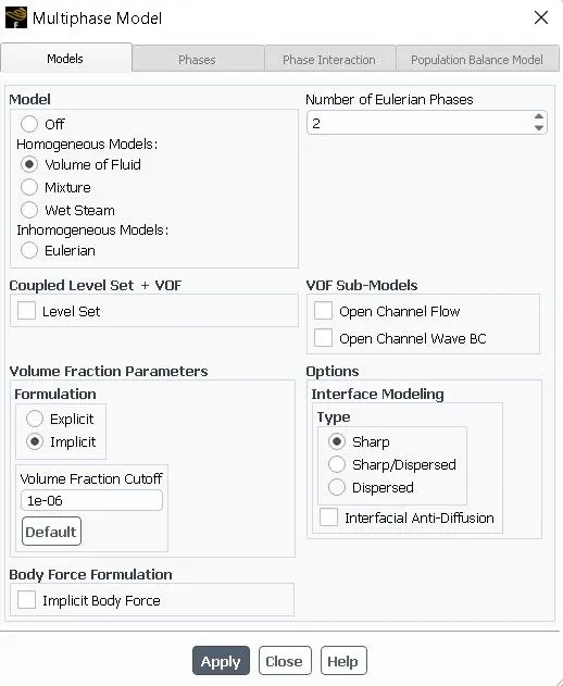
Primary phase – air
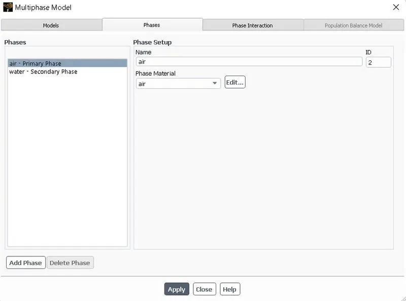
Secondary phase – water
Solving --> select Method=standard > go to Patch --> Phase=Water, Variable=Volume Fraction --> select water_surface=1 > click Patch. Similarly select air_surface=0 > click Patch.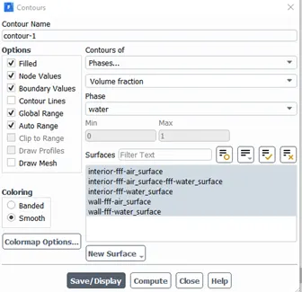
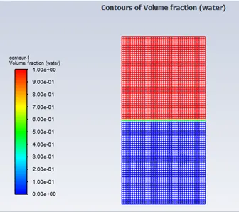
INITIALIZATION:
Standard initialization
Time step size – 0.005s
No. of time steps – 1000
Case 1:
RESULTS:
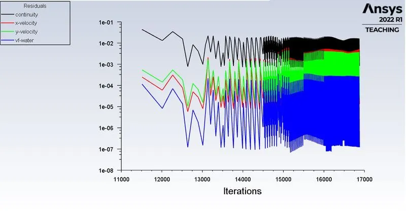
RESIDUAL:
ANIMATION:
youtube link:
It is envisaged from the contour that lower density fluid (Air) is settled on top and the higher density fluid (bottom) is settled at the bottom. This is formed due to instability. This growing instability is known as Rayleigh Taylor's Instability. We could see the formation of bubbles whose position is later replaced by water. The simulation begins with fluids of two phases at a hydrostatic equilibrium state and then Rayleigh Taylor instability is seen at the interference when the lower density fluid pushes a higher density fluid due to which formation of shock waves occurs at the interface. The disturbance at the interface ends with lighter fluid settling up and heavier fluid settling down.
Case:1.2
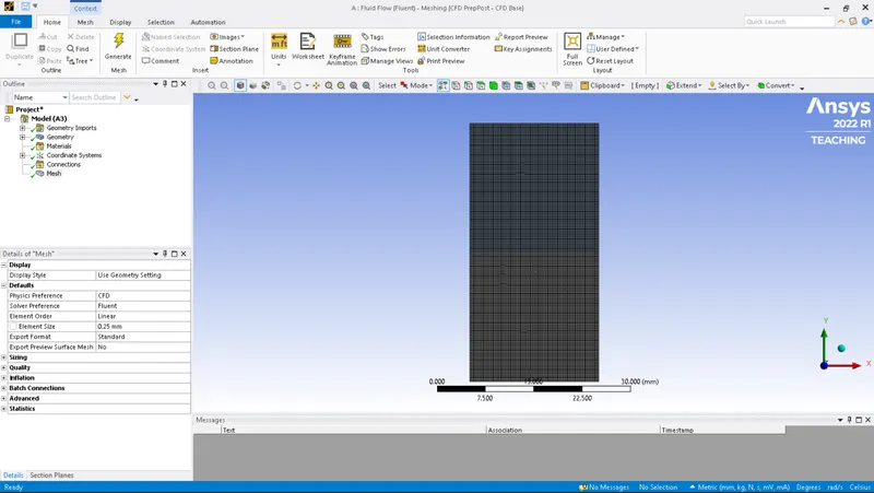
FOR MESH = 0.25MM
A mesh is created for the geometry with a mesh size of 0.25mm. The meshed model will look like the image as shown below
RESULTS:
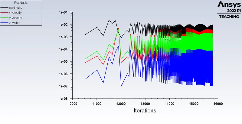
RESIDUAL:
ANIMATION:
youtube link:
Case:2
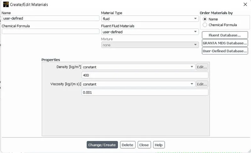
FOR MESH SIZE – 0.25MM AND USER-DEFINED MATERIAL:
MATERIALS:
RESULTS:
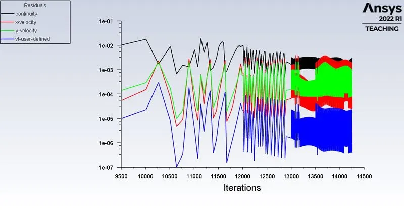
RESIDUAL:
ANIMATION:
youtube link:
is envisaged from the results that simulation begins with fluids of two phases at hydrostatic equilibrium state and then Rayleigh Taylor instability is seen at the interference when the lower density fluid pushes a higher density fluid due to which formation of shock waves occur at the interface. This, in turn, leads to the formation of bubble-like but later it becomes asymmetric, which compresses the heavy fluid around it due to shock waves that push heavy fluid upwards. Later disturbance at the interface ends with lighter fluid settling up and the heavier fluid settling down.
CONCLUSION:
- Rayleigh Taylor instability is observed at the interface of the fluids with different densities under the influence of gravity
- The lower density fluid pushes the higher density fluid above it. The heavier fluid which is water in this case comes at the bottom and replaces the air from the bottom
- Due to the refinement of mesh, we can visualize the instability and irregularities that take place at the interface better.
- In all the cases the lower dense fluid moves into the higher density fluid which causes instability.
- In case 2 we can capture instabilities more accurately due to finer mesh than in case 1.
WHY A STEADY STATE APPROACH MIGHT NOT BE SUITABLE FOR THIS TYPE OF SIMULATION?
the steady state simulation is performed if we are concerned about the final results. In this case, we are more concerned to learn about the irregularities that start developing when we pour highly dense fluid under the gravity effect. So by using a transient solver along with refined mesh we can compute the smooth transition of irregularities that takes place at the interface of the fluids.
DEFINE THE ATWOOD NUMBER:
Atwood number is a dimensionless number in fluid dynamics used in the study of hydrodynamic instabilities in density stratified flows.
A = rho1-rho2/rho1+rho2
Where,
Rho1 – density of the heavier fluid
Rho2 – density of the lighter fluid
FIND OUT THE ATWOOD NUMBER FOR THIS CASE AND EXPLAIN HOW THE VARIATION IN ATWOOD NUMBER AFFECTS THE BEHAVIOUR OF THE INSTABILITY:
Atwood number for the above case is
A = (998.2 -1.225)/(998.2 + 1.225)
A = 0.9975
- When the Atwood number is high, more instability occurs in the fluid, and measuring the spikes of the instability is very difficult.
- When the Atwood number is low the more stable the fluid mixture and measuring the spikes of the instability can be done to some extent because it expresses linearity to some extent.
HOW CAN WE USE THE ATWOOD NUMBER TO VALIDATE OUR SIMULATION RESULT?
SIGNIFICANCE:
- Penetration distance of the heavier fluid into the lighter fluid is given by the formula Agt^2 where g is the acceleration due to gravity and t is the time.
- For A close to 0, RT instability flows take the form of symmetric “fingers” of fluid
- For close to 1, the much lighter fluid “below” the heavier fluid takes the form of larger bubble-like plumes.
For case 1,
A = (998.2-1.225)/(998.2+1.225)
A = 0.9975
For case 2,
A = (998.2-400)/(998.2+400)
A = 0.4278
We see that the lighter fluid air rises up and bubble-like plumes take place. The Atwood number calculated for our result is close to 1. The Atwood number close to 1 signifies the same phenomenon and hence validates our result.