Week 5 - Rayleigh Taylor Instability
AIM-: Rayleigh–Taylor instability with forward gravity effect for two Atwood number.
Theory
Classical Rayleigh–Taylor instability (RTI) is generated at the interface between two different density fluids in the presence of a constant acceleration pointing from the heavy to the light fluid. The interface between the two fluids is unstable to any perturbation with a wavelength larger than the cutoff due to surface tension (for the immiscible case) or mass diffusion (for the miscible case). Thus, small perturbations of the initial interface grow, interact nonlinearly, and lead to turbulence. In most practical cases, RTI manifests itself as an extremely complex process, due to a multitude of factors, among which are large density differences, compressibility, temperature distribution, surface tension and other interfacial phenomena for the immiscible case or mass diffusion for the miscible case, molecular transport variations, geometrical and finite boundary effects, specific plasma and magnetic field properties, and so on. Flows featuring RTI type growth of instabilities can be found in several important natural phenomena and applications, for example, in supernova explosions and X-ray bursts in neutron stars, the solar solar corona, Earth’s oceans, atmosphere, and mantle ,quantum plasma; combustion, inertial, magnetic, or gravitational confinement fusion, sonoluminiscence, etc.
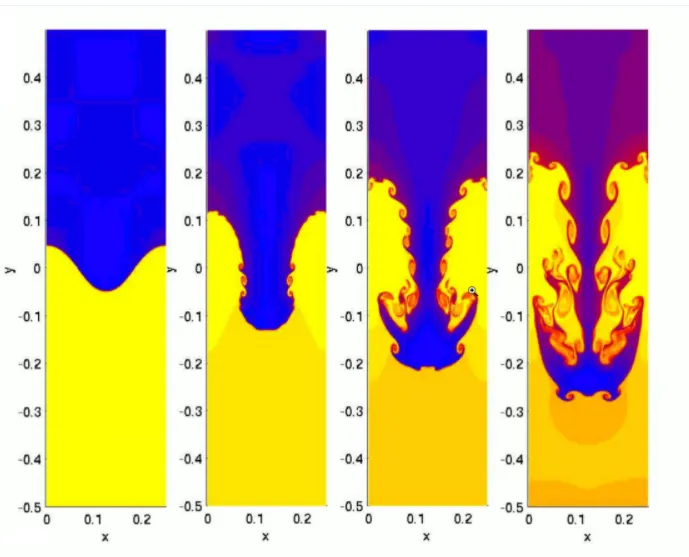
A useful limiting case, which isolates the basic instability from compressibility effects, considers two miscible incompressible fluids with different molar masses. The governing equations can be derived from the fully compressible Navier–Stokes equations under the assumption of an infinite speed of sound or by directly assuming that the two fluids maintain constant densities. We refer to this limit with large molar mass or density ratio (the non-Boussinesq case) as incompressible variable density (VD). Since the acoustic waves are filtered out for the VD equations, K-epsilon at larger resolutions compared to the compressible case become feasible, which implies larger Reynolds and Atwood numbers . Here, we consider RTI in the VD limit.
The strength of the non-Boussinesq effects has traditionally been estimated using the Atwood number, A=ρh−ρlρh+ρl , where ρh,ρl are densities of the heavy and light fluids, respectively. The Boussinesq approximation corresponds to A → 0 and a value of 0.05 is usually taken to define this limit. However, in many practical applications, A ≫ 0.05, for example A ∼ 0.9 in Inertial Confinement Fusion (ICF) and A ∼ 0.85 for hydrogen burning. The development of the instability and the mixing itself are fundamentally different at high and low A. Thus, the RTI mixing layer becomes asymmetric, rougher, and faster growing on the light-fluid side (showing so-called spikes) and smoother and slower growing on the heavy-fluid side (showing so-called bubbles), turbulence intensities are larger in light-fluid regions than heavy-fluid regions and mixing is asymmetric, with pure heavy fluid reaching larger depths from the layer edge than pure light fluid
Governing equations, simulation cases, and numerical method
The incompressible VD equations can be derived from multispecies fully compressible Navier–Stokes equation as the infinite speed of sound limit [14,15], or by assuming that the fluids maintain constant microscopic densities [16,37]. The former derivation uses the energy equation consistently, while the latter simply neglects it in the incompressible limit. For the binary case, these equations are:


The viscous stress is Newtonian with

Eqs. (1)–(2) are the usual continuity and momentum transport equations for compressible flows, with "p" representing only the dynamic pressure component . The limiting process removes the pressure and temperature gradient effects, so that the diffusion operator becomes Fickian in the resulting incompressible equations. Since no other assumption is imposed, the resulting equations are non-Boussinesq. Thus, the density appears in the momentum equations and the divergence of velocity is not zero; the energy equation as well as the species transport equations leads to a formula for the velocity divergence in terms of the derivatives of the density field.
In Eqs. (1)–(3), the independent variables are the time t and space variables, xi , in direction i, ui is the velocity component in direction i, ρ is the mixture density, p is the dynamic pressure and gi are the components of the gravitational acceleration, →g = (0, 0, −g). The kinematic viscosity, ν0 = µ/ρ, and mass diffusion coefficient, D, are assumed constant and uniform in space. Note that, in general, the dynamic viscosity, µ, is a weaker function of density than linear; the assumption ν0 constant ensures a uniform Schmidt number, Sc=ν0/D` throughout the flow.
CFD models based on mathematical analysis of Rayleigh Taylor Instability
Bouyancy Drag model :
It is a model which uses ordinary differential equations to evolve the width of the mixing layer. These models cannot model multiple mixing interfaces, also do not address demixing known as counter-gradient transport, i.e., reduction of total fluid masses within the mixing zone.
BHR Model :
Based on the evolution equations arising from second-order correlations and gradient-diffusion approximations which Uses a mass weighted averaged decomposition, includes full transport equations for the Reynolds stresses, turbulent mass-flux velocity, density fluctuations and the turbulence kinetic energy dissipation rate is the Besnard-Harlow-Rauenzahn also known as advanced version of sinfle fluid models.
K-L model :
The K-L model was proposed by Dimonte and Tipton for describing the turbulent self-similar regime of RT and RM induced mixing.
K-L-a model :
The three-equation model of Morgan and Wickett was developed as an extension to the two-equation K-L model of Dimonte and Tipton by including a third equation for the turbulent mass-flux velocity.
K-L-a-b model : An extension of the K-L-a model by adding an evolution equation for the density-specific volume covariance which reflect the effects of the changes in the density fluctuations
Computation Methodology
N.B- 1. All simulations presented here were performed with the SIMPLE algorithm using 2nd-order Upwind scheme. . To account for the difference in accuracy the grid spacing is refined.
2. Since steady state solver gives significant results at the end state and intermediate results are insignificant and do not hold any physical significance, so it is not worth to use steady state solver when we are keen to ovserve intermediary solution.
3. Atwood number :- Atwood number is a dimensionless number used to describe density difference between two adjacent fluids sharing same interface.
Atwood number=ρ1−ρ2ρ1+ρ2 where, ρ1=densityofheavierfluidρ2=densityoflighterfluid
Atwood number for Baseline and refined case = 998.2−1.225998.2+1.225=0.9975
CASE-1
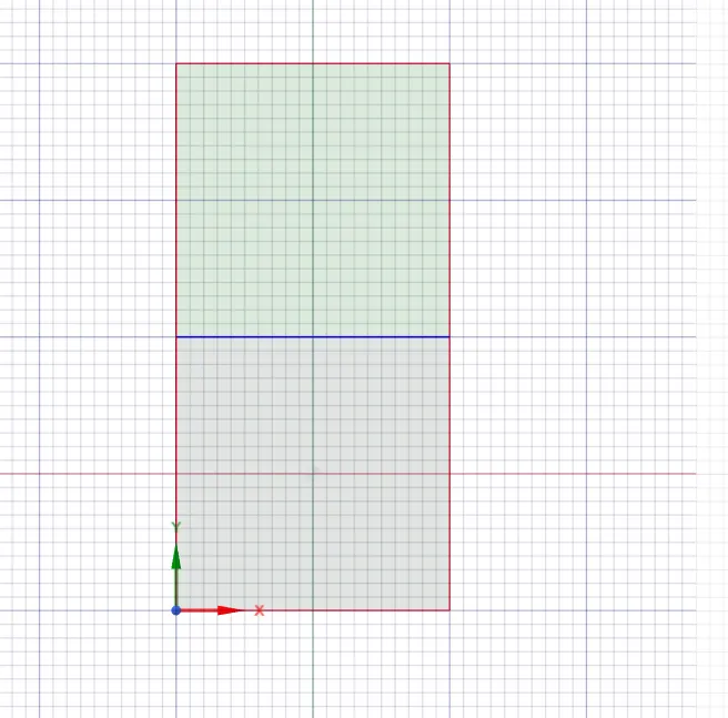
Geometry :
1. Open the geometry section.
2. select the plane and create the geometry according to the givern values.
3. First create the lower voume and extract.
4. Then create the upper volume and extract it.
5. Name both the volumes, upper volume as water and lower one as air.
6. Finally, select the shareprep from workbench for entire volume so they share the interface edge.
Mesh :
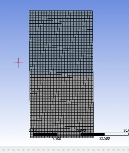
1. Open the mesh section.
2. Go to mesh and edit the elment size according to requirement and mesh the geometry.
N.B- we took Base line mesh for first case.
Setup :
1. Perform Mesh check.
2. Select the transient state approach and add gravity to the problem.
3. Set the viscous model as laminar.
4. Add Volume of fluid as multiphase model and set implicit formulation.
5. Then add materials according to the requirement (we are going to use air and fluid with standard densities and vicosities for first two simulation and water and user defined material for third simulation).
6. Now name both the phases as air and water respectively.
7. Initialize the problem with standard initialization as we are using transient state approach.
8. finally add contour and solution animation and run the simulation for some iteration after setting correct timestep( we are going to run it at 0.005 timestep size and for 1000 timesteps).
Result :
1. Make visible both the upper and lower volume and display variables on both volume.
2. Now create timestep animation and observe the variation with respect to time. We are going to perform simulation on below geometry starting from baseline mesh to refined mesh and refined mesh with user-defined fluid properties.
Case-2
| Element size | Elements | Nodes |
| 0.0002 m | 20000 | 20301 |
| Air | Water | |
| Density (kg/m3) | 1.225 | 998.2 |
| Viscosity (kg/m-s) | 1.7894e-5 | 0.001003 |
Case-3
Atwood number for refined case with user defined fluid properties = 998.2−400998.2+400=0.4278
| Element size | Elements | Nodes |
| 0.0002 m | 20000 | 20301 |
| User-defined material | Water | |
| Density (kg/m3) | 400 | 998.2 |
| Viscosity (kg/m-s) | 0.001 | 0.001003 |
RESULTS
From the figure we can conclude that as we increase the mesh size, we get more detail and accurate result of Rayleigh – Taylor Instability. Since the results show in figure above is final steady-state result, we can understand more about the simulation from their transient response. Animation for all for case has been provided below.
We can use the density of two fluids and calculate the Atwood number for case 1 or 2 and 3 using equation 1. Density of air is 1.225 Kg/m3, water is 99 8.2 Kg/m3 and custom fluid is 400 Kg/m3 using equation 1 and density above we get Atwood number for case-2
Atwood number for Baseline and refined case = (998.2-1.225)/(998.2+1.225)
= 0.9975
For case- 3
Atwood number for refined case with user defined fluid properties = (998.2-400)/(998.2+400)
= 0.4278
Using our understanding of dimensionless number, Atwood number we can we can evaluate our results whether our simulation is correct or not . As stated earlier Atwood number closer to one would have higher density difference creating Bubbles and plumes. For the Atwood number close. To 0 density difference would be smaller creating symmetrical mixing normally a shape of finger initially.
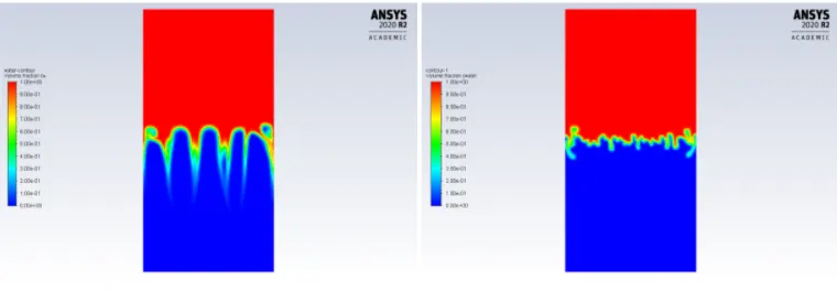
Fig-a Fig(b)
1. Above Figure shows us the initial shape fluid take for different the Atwood number. As we predicted the Atwood number closer to 0 would have symmetrical shape. Not only we see the symmetrical mixing between two fluids for case-3, but we also see the “finger” shape on the figure b.
2. There are many practical application for rayleigh-taylor instability phenomenon from daily uses such as the liquid dispenser or inkjet in printers to supernova explosion and inertial confinement fusion,
Conclusion
1. In conclusion we successfully simulated rayleigh-taylor instability phenomenon, and compare the effect of different Atwood number simulation from available experiment. We compare the simulation result and found that it is the agreement with other rayleigh-taylor instability simulations for Atwood number closer to 1, the density of a fluid on top is much heavier than do it on the bottom that it creats huse baubles and plums under the gravitational field. Also, the penetration of those spike initially reaches much greater height (bottom) due to lighter dense fluid in bottom.
2. On the other hand Atwood number closer to 0 showed symmetrical mixing initially like a shape of finger and penetration of heavier dense fluid not reach larger height. The understanding of this phenomenon has led to many practical applications such as ink jets or will fuel Jets in automobiles.
3. Looking at above videos we can say that refined mesh gives more smooter results. Also we can say that both the fluids settle down faster in coarser mesh and it takes much more time in finer mesh cases.
4. providing correct timestep is important at it gives floating point error if wrong timestep is chosen.
5. Effect of variation in atwood number on above cases :
In First two videos we can clearly see that, the 1st two cases with standard densities of air and fluid has bubble type formation at upper part and spike type formation at lower part at inteference after collapsing and trying to mix. In third video in which refined case has user defined fluid with different density than standard one, forms almost similar bubble like formation on both upper and lower part of interference after collapsing. So we can say that cases with higher atwood number produce bubble type formation at upper part and spike type formation at lower part of inteference. Same way, the case with lower atwood number forms almost similar bubble like formation on both upper and lower part of interference
References:
[1] S. Chandrasekhar, Hydrodynamic and Hydromagnetic Stability, Dover, New York, 1981.
[2] D. Sharp, An overview of Rayleigh–Taylor instability, Physica D 12 (1984) 3–18.
[3] D.L. Youngs, Numerical simulation of turbulent mixing by Rayleigh–Taylor instability, Physica D 12 (1984) 32–44.
[4] W. Cabot, A. Cook, Reynolds number effects on Rayleigh–Taylor instability with possible implications for type-ia supernovae, Nat. Phys. 2 (2006) 562–568.
[5] N.C. Swisher, C.C. Kuranz, D. Arnett, O. Hurricane, B.A. Remington, H.F. Robey, S.I. Abarzhi, Rayleigh–Taylor mixing in supernova experiments, Phys. Plasmas 22 (2015) 102707.
[6] E. Khomenko, A. Diaz, A. de Vicente, M. Collados, M. Luna, Rayleigh–Taylor instability in prominences from numerical simulations including partial ionization effects, Astron. Astrophys. 565 (2014) A45.
[7] S. Gerashchenko, D. Livescu, Viscous effects on the Rayleigh–Taylor instability with background temperature gradient, Phys. Plasmas 23 (2016) 072121.