Week 5.1 - Mid term project - Solving the steady and unsteady 2D heat conduction problem
PROBLEM STATEMENT:
To solve for the 2D Heat-Conduction equation for the steady and unsteady state using the explicit and implicit methods within the given boundary condition.
Solve the equations using various iterative solvers such as:
1. Jacobi-Method
2. Gauss-Seidel-Method
3. Successive Over-Relaxation
Solve for both Steady and Transient state heat of the conduction equation.
The accuracy of the solution obtained through both the explicit and implicit methods should be determined with respect to the 'Tolerance' Value provided.
BOUNDARY CONDITIONS:
Top Boundary = 600K
Bottom Boundary = 900K
Left Boundary = 400K
Right Boundary = 800K
RESULTS & OBSERVATIONS FOR TRANSIENT-STATE 2D HEAT-CONDUCTION EQUATION USING EXPLICIT SCHEME:
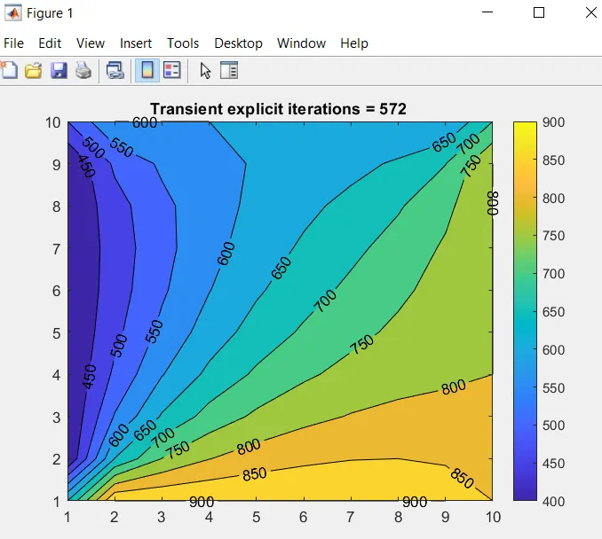
The above plot has a CFL value of less than one as required and hence the Time-Iterations are converging eventually.
If the value of CFL was more than 0.5, then this plot would enter divergence like shown in the image below:-
Tolerance Value for error = 1e−4or10−4
INTRODUCTION :
Numerical solution schemes are often referred to as being explicit or implicit.
When a direct computation of the dependent variables can be made in terms of known quantities, the computations are said to be explicit.
When the dependent variables are defined by coupled sets of equations and either a matrix or an iterative technique is needed to obtain the solution, the numerical method is said to be implicit.
Iterations are used to advance a solution through a sequence of steps from a starting state to a final, converged state. This is true whether the solution sought is either one step in a transient problem or a final steady-state result. In either case, the iteration steps resemble a time-like process.
The principal reason for using implicit solution methods, which are more complex to program and require more computational effort in each solution step, is to allow for large time-step sizes.
A simple qualitative model will help to illustrate how this works.
Let Q be a quantity whose value is Qn+1.
We want to compute at time t = (n+1)dt, in terms of time t = ndt.
i.e., Qn+1 = Qn+dtS, where S is the rate of change in Q.
In an explicit numerical method, S would be evaluated in terms of known quantities at the previous time step n.
An implicit method, in contrast, would evaluate some or all of the terms in S in terms of unknown quantities at new time step n+1. Since new quantities appear on both the left and right sides of the Q-equation, it is said to be an implicit definition of the new n+1 values. Usually, a matrix or iterative solvers must be used to compute the new quantities.
TO SOLVE FOR DEPENDENT VARIABLES, THE FOLLOWING ITERATIVE SOLVERS ARE BEING USED:
1. Jacobi Iterative Solver
2. Gauss-Seidel Iterative Solver
3. Successive Over-Relaxation iterative solver
2D Heat Conduction Equations for Steady and Unsteady states:
STEADY STATE:
∂2T∂x2+∂2T∂y2=0
UNSTEADY STATE:
∂2T∂x2+∂2T∂y2=α∂T∂t

Where,
K1=αΔt(Δx)2
K2=αΔt(Δy)2
n is the time index
(i,j) is the space index
Given:
omega = 1.5;
alpha = 0.05;
dx = dy;
Tolerance Value = 1e^-4 or 10^4
Although we know fact that conduction is a time-dependent phenomenon but eventually it culminates into a steady-state phenomenon with respect to time.
Condition for convergence for the 2D conduction equation is given by Courant-Friedrichs-Lewy Condition. The Stability criterion of a numerical scheme is determined by the way the error propagate while the solution moves from a one-time step to the next in the case of a transient solver. While solving governing equations in the PDE, it forms discretized equations having error terms that should theoretically be minimized or should be oscillated with a damped amplitude so as to gradually minimize the error terms as one move forward in time, we define this important criterion as the CFL Number which stands for the Courant-Friedrichs-Lewy Condition which is essential for convergence of a solution by the method of finite differences. It also sets the condition that if the time=step of the problem is larger than a specific value the solution of the finite difference equation becomes impossible by some solvers.
The condition for the 2D case is given below:
C=α⋅(1(Δx)2+1(Δy)2)⋅Δt
Where,
α= Thermal Diffusivity(Units = m2s−1)
Δx=Δy= Number of grid points in the x or y direction(Units = m)
Δt = Time-Step
Where C≤Cmax=0.25 for convergence. Here Cmax= 0.25 is for the explicit.
Implicit solvers are unconditionally stable and are less sensitive to numerical instability so they can tolerate a much larger value of C where an explicit solver might fail.
STEADY-STATE ANALYSIS:
MATLAB CODE TO SOLVE FOR 2D HEAT CONDUCTION EQUATION FOR STEADY-STATE :
MATLAB CODE EXPLANATION:
1. Firstly, we are taking two inputs nx & ny, both of which are being assigned with the value of 10.
2. Then, we're using both nx and ny to create a 2D matrix of 10x10 order using the 'ones' command.
3. We're then adding the respective boundary conditions for temperatures of all the faces which are provided in the challenge.
4. Now, we're mapping the values of the boundary conditions for their respective rows and columns as shown in the image below.
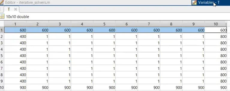
5. We can see from the above image that the values of boundary conditions are overlapping over one another in the case of the first and last columns.
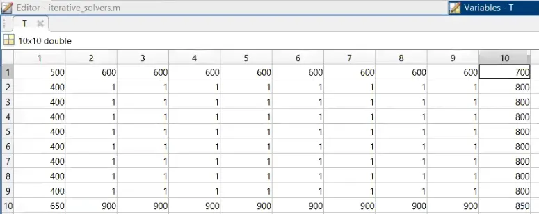
6. We're then refining the edges by taking the average from it by adding both the top and bottom node's values and diving it by 0.5 as shown in the image below.
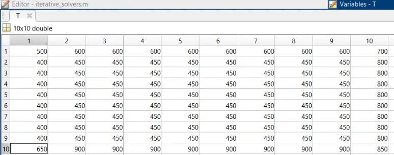
7. Now, we know that the nodes present inside the boundary conditions cannot be 1 because it has to be more than 400 and less than 900 those two being the minimum and maximum values from the matrix. So, we'll provide a proper guess value of 450 by multiplying 450 with the 'ones' command in our previous statement which was used to create the matrix firsthand.
The result is shown in the image below:
8. Everything in the code is stated in a way that will enable it to adapt to various inputs by itself and we wouldn't need to make changes for each of the values individually.
9. Now that we're done with the formulation of the domain to work with, we can now implement various iterative solvers such as Jacobi, Gauss-Seidel, and Successive over-relaxation methods to reach convergence.
10. Before starting with the iteration process, we're storing the values of 'T' inside 'Told' and 'T_initial'.
11. We're taking our error value as 9e9 and tolerance value of error as 1e-4. Both of these values are essential for the convergence process to happen.
12. Now, we're introducing a while loop with the initialization statement of 'while error is bigger than tolerance'. i.e. while(error>tol).
13. As we know that we cannot run our iterations on the boundary conditions hence we will take a for loop to compute from the 2nd node of the second row to the 2nd node of the ninth row, so 'i' will be from 2 to nx-1.
Under that, we'll state another for loop which will compute from the 2nd node of the second column to the 2nd node of the ninth column, and hence 'j' will be from 2 to ny-1.
We have to keep in mind the directions of rows and columns here are the opposite of the cartesian coordinate system.
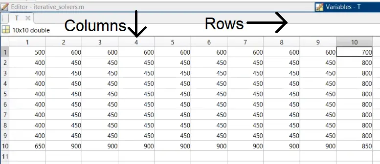
This way, for each value of 'i' it'll compute all the corresponding values of 'j' from that row, and then when 'i' gets incremented again, it'll compute the corresponding value of 'j' for that row and so on.
14. If we see the discretized equation for steady-state, it is derived as T = 0.25*[Horizontal Component+ Vertical Component] which is given as:
T(i,j) = 0.25*(Told(i+1,j) + Told(i-1,j) + Told(i,j-1) + Told(i,j+1));
15. As we're following Jacobi Iteration Method here so we have to take values from the 'Told' matrix and not the current matrix 'T'.
16. Now, in order to bring the iterative process to a stop we need the solutions to converge. It'll converge only when the value of error has decreased to such as extent where it is very close to the provided tolerance's value.
17. So now, we have to compare the two matrices 'T' and 'Told' to check the degree of error. Remember, the error is a single value and not a 2D matrix but both 'T' and 'Told' are 2D matrices. hence we have to compare the maximum value from each matrix with one another in order to check the error value.
18. To do so, we're implementing the 'max' command in order to compute the maximum value of error from each matrix which we can then compare with the given tolerance's value.
It is stated as: error = max(max(abs(T-Told)));
19. After that we'll update the value of 'Told' into the 'T' matrix. We have to update this after the error has already been compared and not before.
20. Now we're introducing an iteration counter named 'jac_iter' which will count the number of times Jacobi's iterations have occurred.
21. In the image below we can see how the values of various nodes within our boundary have changed as the iteration process took place.
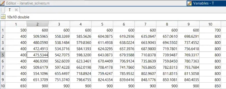
22. We can notice that the values of nodes are within the stated boundaries and are increasing towards boundary conditions with higher values and are decreasing towards the boundary conditions with lower values.
23. Now we can plot the above using the 'contourf' command which gives us a 2D view of the iterations for T with colors. Here 'ShowText' command is also used which enables us to view the index of iteration which is currently running.
24. We're then using the 'pause' command with the value of '0.05' which will visualize the whole iteration process to us in real-time.
25. We're now using another command known as 'colorbar' which will help us to make sense of the plot by showing us the relation between numerical values and the colors represented in the plot after the solution has converged.
26. Another thing that we'll notice is when we view our plot after convergence, the values will be inverted for the top and bottom boundary conditions due to the previously used 'contourf' command. So, in order to fix this, we're now introducing the 'flip' command as 'flipud' where 'ud' stands for up & down, and hence we're inverting the top and bottom boundary conditions for the plots.
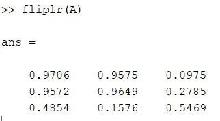
An Example of the 'flip' command for up & down, as well as left & right, is as follows:
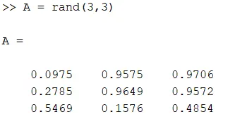
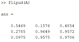
27. Now, we're going to plot the title for the plots and we'll do it in such as way so that it'll continuously update the value of iteration count for each time it executes a respective plot from the Jacobi Iteration Method.
28. Now that we have created a 2D solver for Jacobi Iterative Method, we will copy-paste the code from Jacobi's section and utilize it to create Gauss-Seidel and SOR solvers.
29. The only difference between Jacobi's Solver and GS's Solver is that in the case of GS, we're using the values from our current matrix 'T' and not 'Told' for i-1 and j-1.
30. We'll also create a new variable named 'gs_iter' to keep track of the GS iterations.
31. We also need to reinitialize the value of our matrix 'T' to the nascent state of the 'T_initial' matrix as we'll need a fresh matrix to utilize for GS-iterations.
Also, we've to reset the value of error to 9e9 because our error value has decreased significantly from our previous operation.
32. The number of iterations that will occur in the GS Method before the equation is converged will be lesser than the number of iterations in the Jacobi Method because here we're not using the previous values and only the current computed value which then minimizes the length of the operation to reach convergence.
33. Now we'll use the Successive over-relaxation(SOR) iterative method. Firstly, we'll state a SOR iteration counter named 'sor_iter' which will again start from 0.
34. The formula for the SOR method is (1−ω)Told+ ω⋅TGS
35. So we have the GS formula of
T(i,j) = 0.25*(Told(i+1,j) + T(i-1,j) + T(i,j-1) + Told(i,j+1));
We'll need to multiply TGS with ω& we have to subtract 1−ω and then multiply it with previous iteration's matrix.
36. Now, we'll rename T(i,j) from the previous GS formula to TGS(i,j) and we're going to say T(i,j) is equal to (1−ω)⋅Told(i,j)+ω⋅TGS(i,j).
37. Value of omega(ω) is set as 1.5. Basically, whenever we're giving the value of omega, it should be between 0-2. If it's between 1 then it is termed as under-relaxation and if it's between 1-2 then it is termed as over-relaxation. If we use any value which is greater than this value then the solution will experience divergence.
38. We have to reinitialize the matrix and the error value each time we switch iterative methods.
RESULTS FOR STEADY-STATE 2D HEAT-CONDUCTION EQUATION:
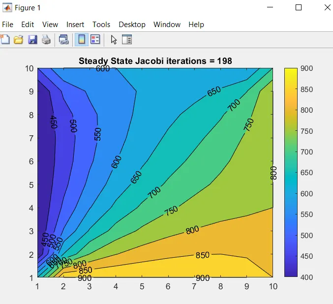
1. JACOBI ITERATIVE METHOD:
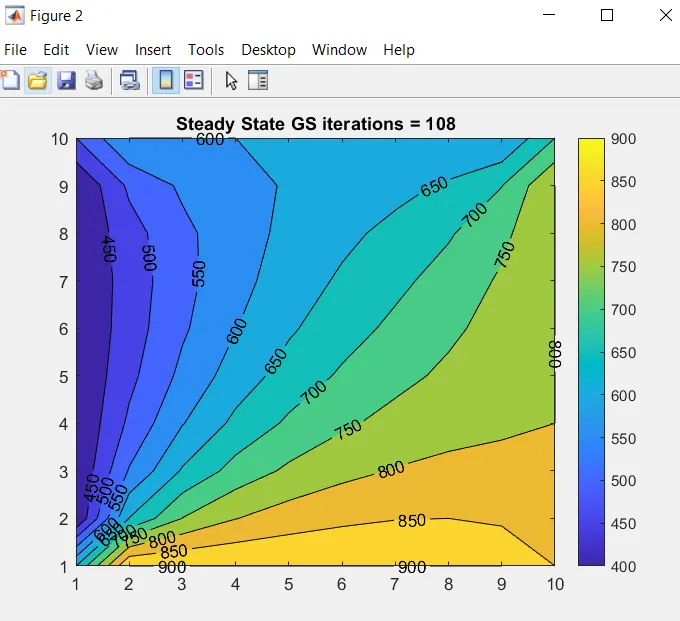
2. GAUSS-SIEDEL ITERATIVE METHOD:
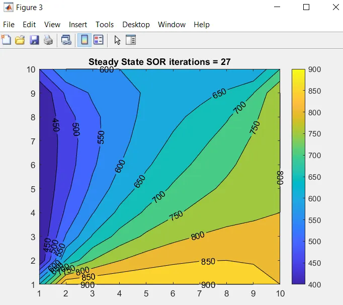
3. SUCCESSIVE OVER-RELAXATION ITERATIVE METHOD:
OBSERVATIONS:
No. of iterations required in Jacobi's Iterative Method: 198
No. of iterations required in Gauss-Seidel's Iterative Method: 98
No. of iterations required in Successive Over-Relaxation's Iterative Method: 27
As we can observe from the above plots that all these methods give rise to the same solutions but the number of iterations required to reach the convergence value is different for each method.
Hence, we can come to the conclusion that using different iterative solvers won't give us different results as the equation on which the methods are used remains the same.
TRANSIENT-STATE ANALYSIS FOR EXPLICIT AND IMPLICIT SCHEMES:
We'll start with the Transient-state for Implicit scheme.
Working principle of the Implicit Scheme:
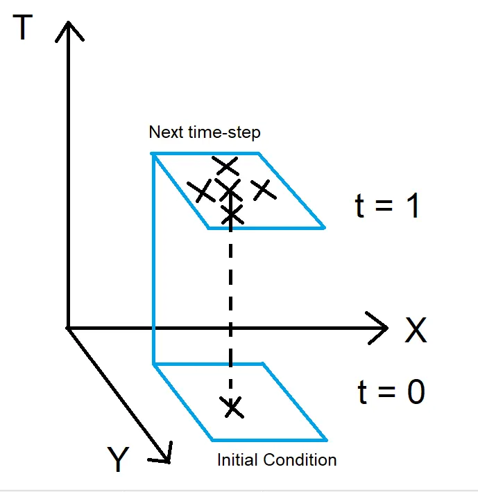
1. We have a matrix with the boundary conditions and the initial conditions at time t = 0 as shown in the above image.
2. Now, if we need to calculate the value of a node in the next matrix at time t = 1, the implicit formulation requests the value of that particular node from its previous position at the first matrix which is at the time t = 0.
3. Now, if we want to calculate the values of the neighboring nodes of the previous node at t = 1, we have to consider them as unknowns as here only the value of the node at a time, t = 0 is known to us.
4. So, we have 5 unknowns right now.
5. When we try to write the equations for all the terms, we get a series of unknowns like this in such a way that we have a system of equations for every node.
6. So it results in the formulation of a system like this one: A*X = B
7. Here A is the 'Coefficient', B is the 'Boundary Conditions' and X is the 'Unknowns'.
8. This is what we are trying to solve iteratively same as in our steady-state code by using various iterative solvers like Jacobi, GS, and SOR.
9. Here, iterations take place at each of the time steps. To find out the values of nodes at each matrix for varying time steps we have to write code so that the current matrix considers the value of its nodes from the previous matrix at the previous time step and takes the matrix further upwards in time.
10. We can consider the number of time steps to be 'nt'. So we have to use a criterion to denote the number of time steps it will go up for.
11. We have to then calculate the number of iterations it takes for the equations to converge at each time step.
MATLAB CODE FOR TRANSIENT-STATE OF 2D HEAT-CONDUCTION EQUATION THROUGH IMPLICIT SCHEME:
MATLAB CODE EXPLANATION:
1. We'll use the same domain as used in steady-state with slight modifications.
2. Values of nx, ny, 'T' matrix, Face Temperatures, Boundary-Conditions, Edge Refinement will be the same.
3. We'll provide the new equation for the transient-state of the heat-conduction phenomenon in the code which is derived as follows:
= ∂T∂t=α⋅[∂2T∂x2+∂2T∂y2]


Tˆp(n+1)=Tˆp(n)(k1⋅(H)+k2⋅(V)1+(2⋅k1+2k⋅2)
Where H = Horizontal Component & V = Vertical Component

4. Hence, the new equation is given as: (1+2*k1+2*k2)^-1*(Tprev(i,j) + k1*(Told(i-1,j) + Told(i+1,j)) + k2*(Told(i,j-1) + Told(i,j+1)));
5. As we're using the Jacobi Method at first hence we're using the 'Told' value in the above equation.
6. Timestep value will be stated by the variable 'dt' whose value will be considered as dt = 1e-2.
7. Grid-spacing value will be stated by the variable 'dx' & 'dy' whose value will be considered as dx = 1e-2 & dy = 1e-2 respectively.
8. The value of Thermal Diffusivity will be stated by the Variable alpha whose value will be considered as 0.015 which is a very realistic value as we'll find many materials with such a value of thermal diffusivity and hence, we're considering this value for observational purposes and to find out the number of iterations the equation will need to reach convergence.
9. Here, we have to maintain 3 different matrices, 'T', Told, and Tprev and hence we'll add Tprev to our current equation.
10. When we're going forward in sense of timesteps, Tprev will store the value of our previous matrix.
11. In order to know if Told has converged or not we're taking the difference between Told and T for which we'll use the variable 'error'.
12. Also, to know whether T and Tprev have converged or not we're taking the difference between them for which we have introduced a new variable known as 'conv'. Its value is also stated the same as the error which is 9e9.
13. This will eventually tell us the duration for which we have to keep marching the time steps forward.
14. The calculations are happening inside the 'Space Loop' and the values of T are getting stored as Tprev.
15. So now, we also need to take into account how many times iterations have taken place. For that, we'll introduce a new variable named 'jac_time_iter' which will store the values of time steps and we're going to put it in incrementing order.
16. So the point up to which the error is greater than tolerance the space loop keeps the iteration going and when it finally comes closer to the value of the tolerance, it converges.
17. Also, after each time the space loop completes its cycle the value of error has to be reinitialized to 9e9 otherwise it'll not enter the time loop again and our equation will not experience the time-marching process.
18. In the case of the Steady-State equation we're directly viewing the end results while in the case of Transient-State we're viewing the intermediate solutions between various time-steps.
19. We'll then use the code of the Jacobi Method to create Gauss-Seidel and SOR solvers and before starting any new method we must reinitialize the values of T, Told & Tprev, 'error', and 'conv' so that it'll not interfere with the results of one another.
20. So, in the case of Gauss-Seidel, firstly, we'll introduce a Gauss-Seidel Time-Iteration. Also, we're only using the 'T' matrix here and not Told in the case of i-1 and j-1.
21. We'll use the current code of GS iterations to create a SOR solver and make changes accordingly.
RESULTS FOR TRANSIENT-STATE 2D HEAT-CONDUCTION EQUATION USING IMPLICIT SCHEME:
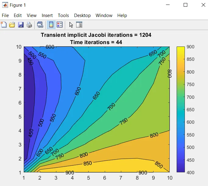
1. JACOBI ITERATIVE METHOD:
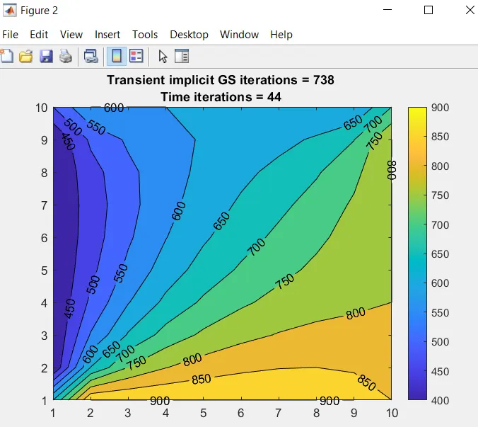
2. GAUSS-SEIDEL ITERATIVE METHOD:
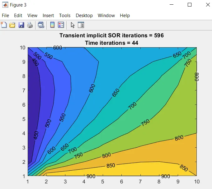
3. SUCCESSIVE OVER-RELAXATION:
OBSERVATIONS:
1. No. of space iterations till it reaches convergence and No. of time iterations till it reaches convergence for each method:
No. of Iterations till convergence in Jacobi = 1204, No. of time iterations till convergence in Jacobi= 44
No. of Iterations till convergence in Gauss-Seidel = 738, No. of time iterations till convergence in Gauss-Seidel= 44
No. of Iterations till convergence in SOR = 596, No. of time iterations till convergence in SOR= 44
2. We can clearly see from the above results that the time iterations are the same for each and every method but the number of iterations taken to reach the value for convergence is going down eventually as we go from JACOBI to GAUSS-SEIDEL and finally to SOR.
We will now move on to the Transient-State for Explicit Scheme.
WORKING PRINCIPLE OF AN EXPLICIT SCHEME FOR A TRANSIENT-STATE 2D HEAT CONDUCTION EQUATION:
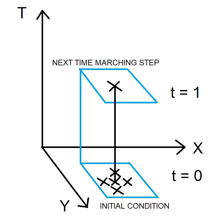
1. The Explicit-Scheme tells us that in order to find out the value of the node at the next time step we need the value of that node from its previous matrix and the value of its neighboring nodes.
2. The entire matrix is already known to us here and we just have to increment the value of our time.
3. We don't require any iterative solvers here as we can reach convergence just by going up in time.
4. The only thing we should be concerned about here is how long we need to increase our value of time.
5. We can estimate that by using a convergence variable which will enable us to subtract the temperature matrix at the time, t = 0 and t = 1, and so on so that we can compare the value we got after subtracting it with one another and compare it with the value of convergence to determine whether or not it has reached convergence.
6. The only iteration present here is for time-iteration.
7. Discretization:
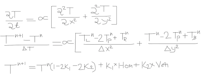
8. We're then going to state our discretized equation inside the time loop and we're using only Tprev.
9. We don't have a value of error here but rather have a convergence value to compare the plots with.
10. We're also introducing a new variable named 'time_iter' which will count the number of times our time iteration's value has been incremented.
11. We have to implement an additional parameter called CFL which stands for Courant-Friedrichs-Lewy. CFL is given as k1+k2 here.
12. Implicit conditions don't require the CFL parameter. The value of CFL should be less than 0.5 for a 2D system of equations.
13. Here, the value of our CFL is 0.1600 which satisfies the above-mentioned condition.
14. If the value of CFL increases more than 0.5, it enters divergence instead of convergence.
MATLAB CODE FOR TRANSIENT-STATE OF 2D HEAT-CONDUCTION EQUATION THROUGH EXPLICIT SCHEME: