Week 5 - Rayleigh Taylor Instability
Rayleigh Taylor instability:
From the Newton law of viscosity, we know that even the fluid cannot resist the slightest shear force. Density is one of the main property of the fluid which the shear force can incorporate with it.
Depending upon the density we have lighter fluid like water etc and denser fluid like mercury, oil, honey etc.
Lord Rayleigh observed that when two liquids i.e lighter and heavier fluids are mixed together where the denser fluid is top on the lighter fluid, due to the gravity and the density variation the interface of the liquid is not stable. (i.e water suspended on the oil)
So, the instability of the interface between the different densities of fluid when the lighter fluid is accelerated towards the heavier fluid is known as RAYLEIGH TAYLOR INSTABILITY.
Types of instability and some practical CFD models that have been based on the mathematical analysis of Rayleigh Taylor waves:
Ritchmyer-Meshkov instability:
The Ritchmyer-Meshkov instability arises when a shock wave interacts with an interface seperating two different fluids. It combines compressible phenomena, such as shock interaction and refraction, with hydrodynamic instability, including non-linear growth and subsequent transition to turbulence, across a wide range of Mach numbers.
Plateau- Rayleigh instability:
The Plateau- Rayleigh instabilit, often just called the Rayleigh instability, explains why and how a falling stream of fluid breaks up into smaller packets with the same volume but less surface area. This fluid instability is exploited in the design of a particular type of ink jet technology where by a jet of liquid perturbed into a steady stream of droplets.
Kelvin-Helmholtz insatbility:
The Kelvin-Helmholtz insatbilitycan occur when there is velocity shear in a a single continous fluid, or where there is a velocity difference across the interface between the two fluids. An example is a wind blowing over water. The instability manifests in waves on the water surface. More generally, clouds, the ocean, saturn's bands and the sun's corona show the instability.
Simulation :-
In the Rayleigh Taylor instability the idea we have a dense fluid at the top and light fluid at the bottom and that interface is going to be unstable when gravity is present and this is going to result in lot of cool looking flow pattern but the question is why we are doing this? well we are doing this to learn two things one we are going to be learning something called as the volume of fluid method which is an important technique that is used to simulate two phase flow and that is why we are working on this particular problem and this analysis is going to be 2D and hence the whole process is doing to be fairly straightforward.
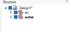
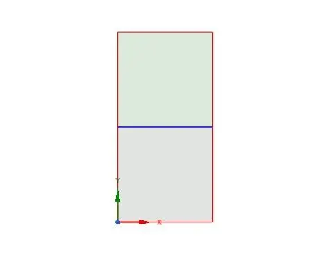
First of all i am going to create a square and dimension is 20mmx20mm and then i used pull tool to create a surface of this and we have to remember this is 2D analysis and onces we have the surface and i am going to move to a new component and this is going to be called as 'air' and
Next i am going to create new component by the clcik on the 'design' as the name 'water' and for water i am creating a new sketch and create a square box with same dimension 20x20mm and used pull tool to make this surface.
Next i am going to 'workbench' and then move to 'share' and select those 2 components and click on and in the left hand side we can see that in the preview boxes the icons are modifield and share Topology enable automatically.
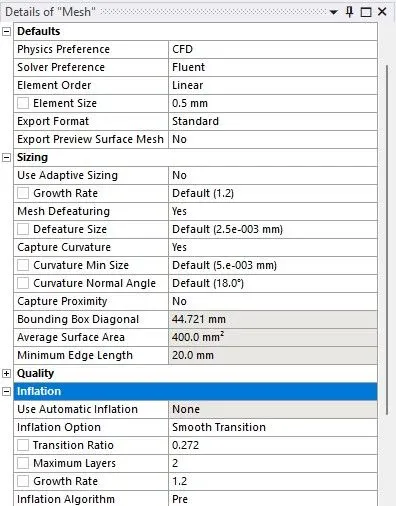
So in the meshing are provide element size is about 0.5mm and generate a mesh
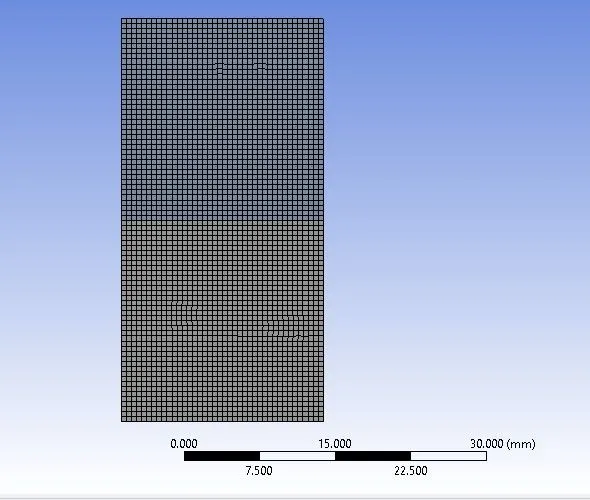
Now,to update the mesh and launch Ansys fluent with 4 parallel processor.
In this we are using 'Transient state' simulation because we want to see how these interfaces collabes as a function of time.
We need 'gravity' enable and provide the value of y as -9.81 why negavtive because y is in the oppposite direction.
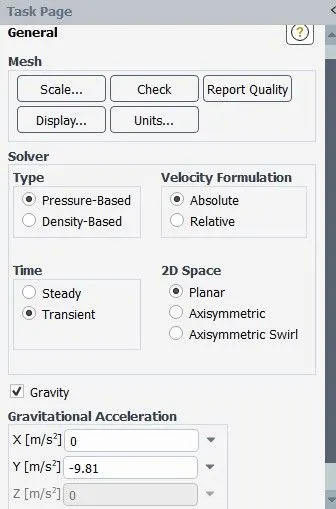
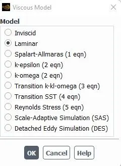
So let's go to Setting-up physics here i am used 'laminar' flow because velocity should be very much slow.
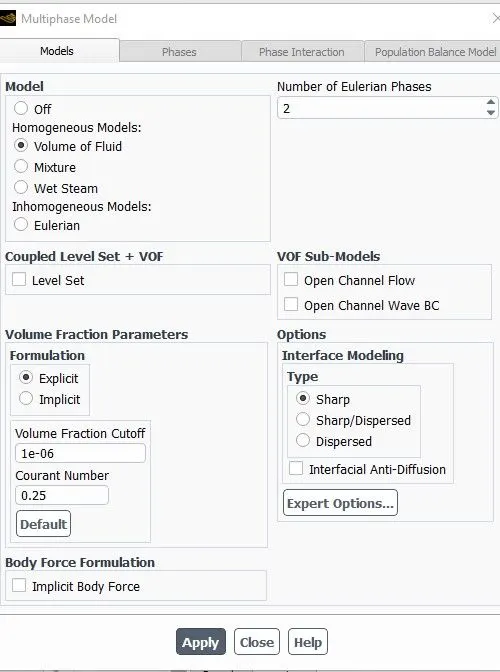
Enable the multiphase model and we are interested in doing 'volume fluid method' where we have 2 Eulerian Phases, the first phase represent as 'air' and second phase represent as 'water'
So in the Material recall fluent database here i am going to import/copy the water
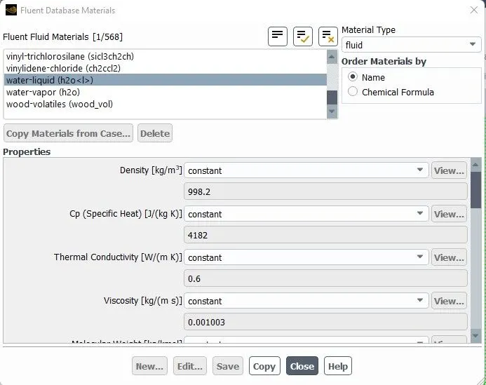
and now air and water are showing in the edit and material box.
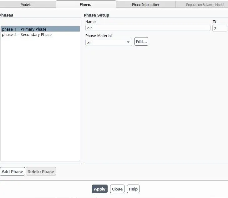
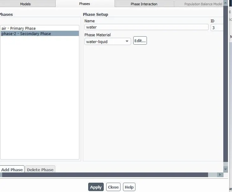
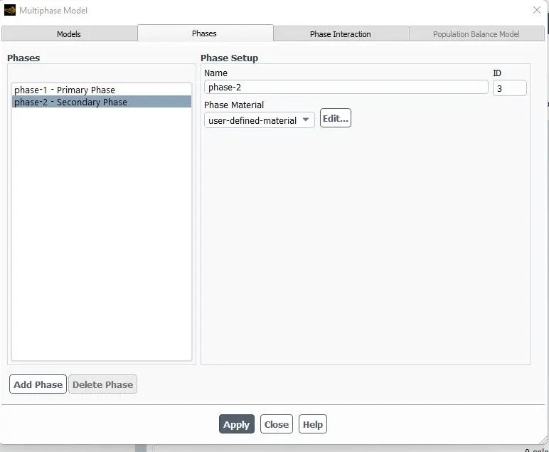
So in the multiphase Model we have 'Phases' and phase 1 is primary phase and it can 'air' and phase 2 is secondary phase and it needs to be a 'water'
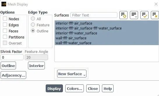
Now go to Domain and let's check it out the Mesh surfaces.
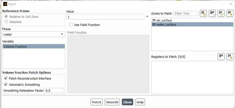
So move to the solving/Solution section and select the standard initialization and there is one of the option is 'Patch' and select the phase as water and put it into a Volume fraction and select the water surfaces and i am here put it in a value of '1' and then patch it.
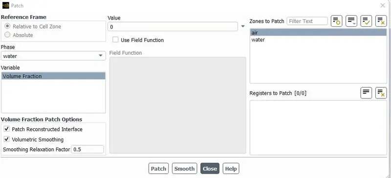
and then i am going to select the air_surface zone and give the value as '0'
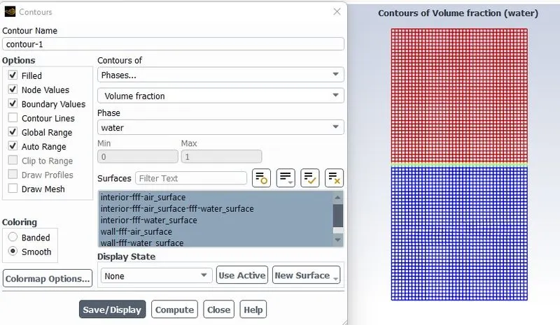
Now create a new contour and select the respective values as shown
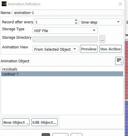
I am going to make now Solution Animation plot for contours and i want it for every time step.
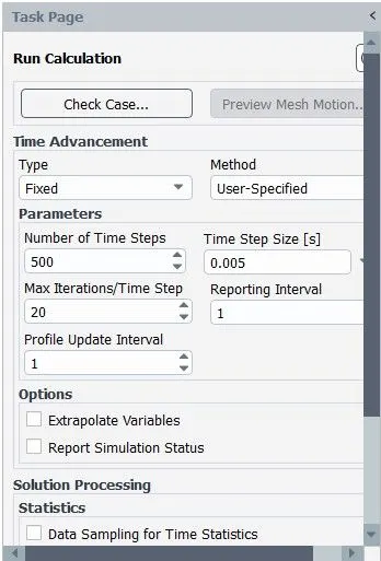
Hit on the RUN calculation by provide appropriate value of Transient model such as 0.005 time step size and 500 time-step.
Case 1 : Mesh element size : 0.5 mm (Baseline mesh {Air-water}):
Mesh
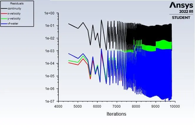
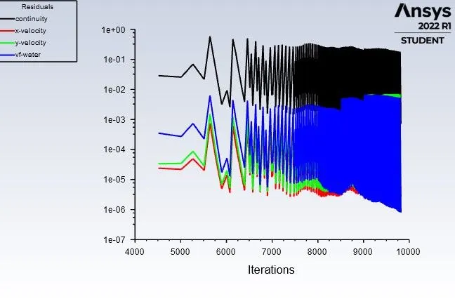
Residual
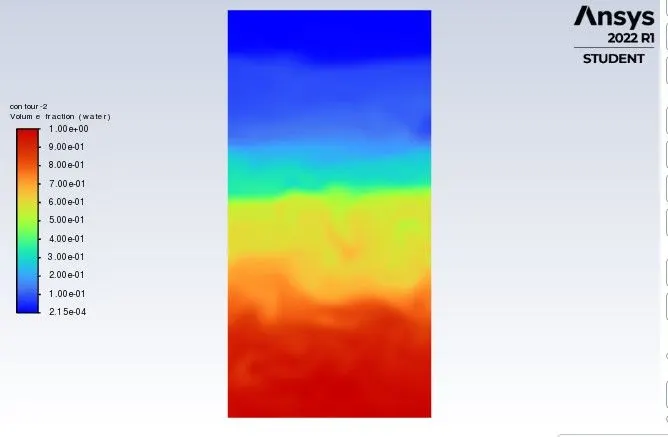
Volume Contours
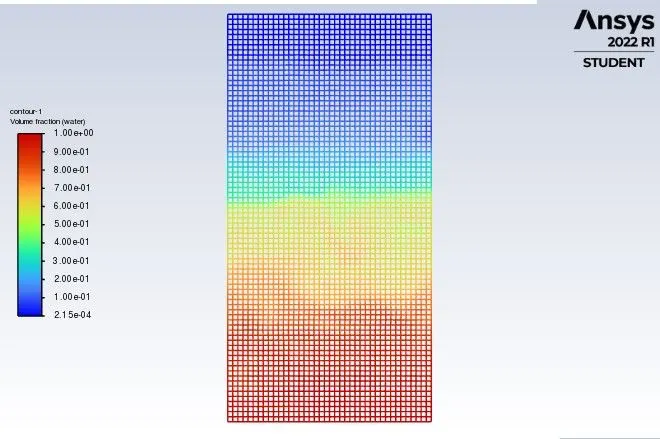
Case 2 : Mesh element size : 0.3 mm (Refined mesh {Air-water}):
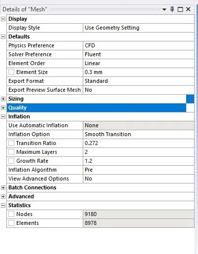
Mesh
Residuals
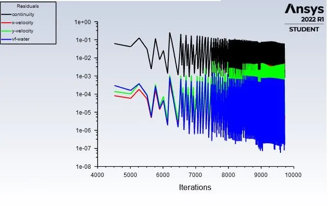
Case 3 : Mesh element size : 0.5 mm (Baseline mesh {Water and user-defined material}):
i was tried with refined mesh for 0.1 mm so many times but the system hang up, anyhow it took 5-6 days but i was going to happened so finally i come up with baseline mesh.so we can see below all the configuration :-
Mesh
Multiphase for user-defined material
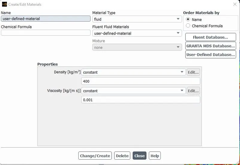
Edit-material
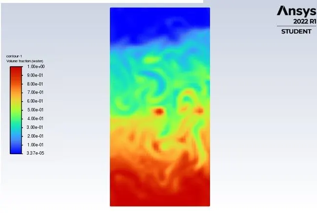
Volume contour
Residuals
Post-processing
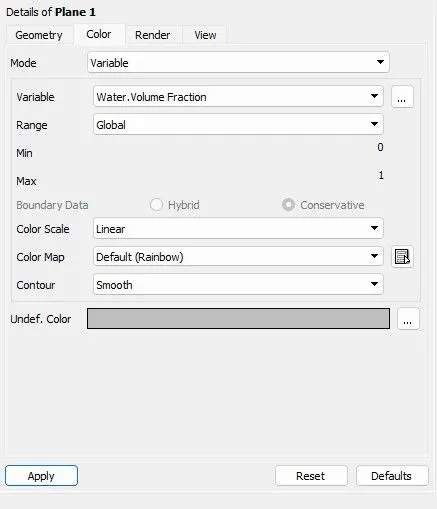
Create a plane and choose the variabel as Water volume fraction.
Now hit on the movie button in the status bar and below window going to be appear
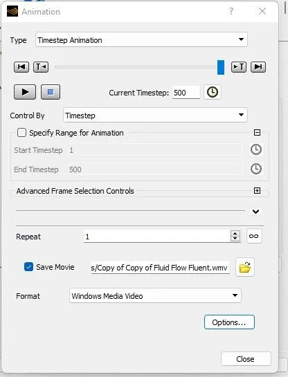
Now let's run and save the animation and upload it to the youtube platform.
Atwood Number (A)
It is a dimensionless number used in the study of hydrodynamic instabilities in density stratified flows. It describes the density difference between two adjacent fluid with a common interface.
`A = {rho_1 - rho_2}/{ rho_1 + rho_2}`
where,
`rho_1` = denisty of the heavier fluid
`rho_2` = density of the lighter fluid
For positive Atwood number, the interface is unstable, and for nagative Atwood number interface is stable.
For Atwood no. close to '0', Rayleigh Taylor instability flow takes the form of symmetric 'fingers' of the fluid.
For Atwood no. close to '1' the much lighter fluid below the heavier fluid takes the form of larger bubble-like plumes.
`rho_1` = denisty of water = 997kg/m^3
`rho_2` = density of air = 1.225kg/m^3
`A = {rho_1 - rho_2}/{ rho_1 + rho_2}`
A = (997-1.225)/(997+1.225)
A = 0.09
Atwood number is an important parameter in the study of Rayleigh-Taylor instability. In this, the penetration distance of heavy fluid bubbles into the lighter fluid is a function of acceleration time scale.
A small density difference,At <0.1 , up-welling (bubbles) and down-welling(spike) disturbances from a symmetrical mixing region that expands away from the initial position of the density interface and is based on the reviewers experiences rather than on any extensive reported study.
As the Atwood number increases, the spike penetration is greater than that of the bubble.
RESULTS :- By comparing all the case i came into conclusion that as we go on decreasing the mesh size the mixing of both fluid will get more smooth and realistic to physical case, More finer the mesh greater the smoothness in mixing has been achieved.
The Steady state analysis can not be used in this case because in th steady state we focus only on the End results. But here in the senario we have to carried out results and record it for each time step so that we can observe the intermidiate behaviours of fluids.That's why transient analysis is must in the case to capture the intermidiate relations and behaviour of mixing fluid.
Animation Video
1. For Water-Air Fluid flow Fluent for Meshing size 0.5mm
2. For Water-Air Fluid flow Fluent for Meshing size 0.3mm
3. For User-defined material flow Fluent for Meshing size 0.5mm
https://youtu.be/a6CfjD4Nvuk