Week 5 - Rayleigh Taylor Instability

Objectives:-

1. What are some practical CFD models that have been based on the mathematical analysis of Rayleigh Taylor waves? In your own words, explain how these mathematical models have been adapted for CFD calculations.
2. Perform the Rayleigh Taylor instability simulation for 2 different mesh sizes with the base mesh being 0.5 mm. Compare the results by showing the animations( Attach them from your google drive). Observe the differences in the animation and explain the effect of mesh size on simulation. Also, explain why a steady-state approach might not be suitable for these types of simulation.[ Choose Air and Water for this simulation]
3. Run one more simulation with water and user-defined material(density = 400 kg/m³, viscosity = 0.001 kg/m-s) for refined mesh.
4. Define the Atwood Number. Find out the Atwood number for both the cases and explain how the variation in Atwood number in the above two cases affects the behaviour of the instability.

Introduction:- The Rayleigh-Taylor instability is an instability of an interface between two fluids of different densities which occurs when the lighter fluid is pushing the heavier fluid.

Examples include the behaviour of water suspended above oil in the gravity of earth and mushroom clouds like those from volcanic eruptions and atmospheric nuclear explosions in which expanding core gas is accelerated into denser shell gas instabilities in plasma fusion reactors and inertial confinement fusion

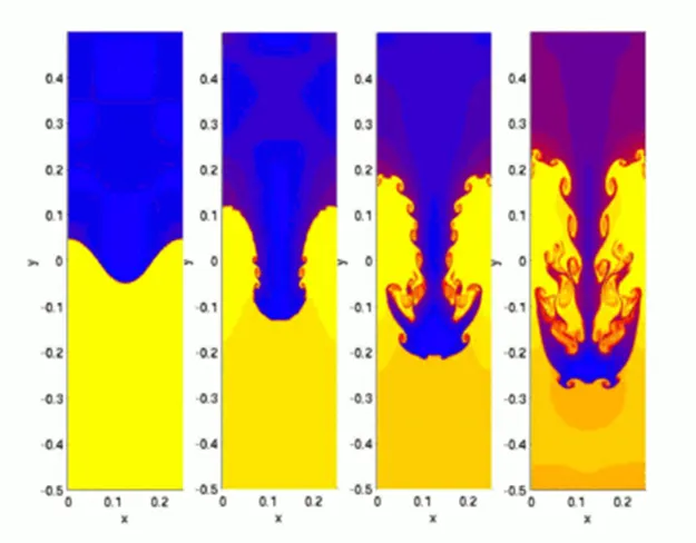
Practical CFD models of Rayleigh Taylor Instability

Some popular models of Rayleigh-Taylor instability are as follows:

Single-Fluid model

A typical approach used for the analysis of two-phase flows is a mixture model, i.e the individual fluid phases are assumed to behave as a flowing mixture described in terms of the mixture properties. The applied single-fluid model is a five equation model consisting of mass, momentum and energy equations for a vapor/liquid mixture and two equations describing the formation and growth of the liquid phase.

Two-Fluid Model

In the two-fluid model, separate sets of the governing equation for the vapour and liquid phases have been used. The interaction between the droplets and the heat exchange between the liquid phase and the solid boundary are not modelled here as well. Additionally, the velocity slip between vapor and the liquid phase is in this model taken into account

Turbulence Model

Turbulence models are needed to predict the average mixing behaviour in flows that are on average one or two dimensional. The approach to the construction of tile turbulence model is guided by the experimental behaviour. The equations governing turbulent flows can only be solved directly for simple cases of flow. For most real life turbulent flows, CFD simulation use turbulent models to predict the evolution of turbulence. These turbulence models are simplified constitutive equations that predict the statistical evolution of turbulent flows.

Why a steady-state approach might not be suitable for these types of simulation

Steady state simulations are run for equilibrium flows where the final state of the flow is required. Transient state analysis is run to understand the variation in the flow at every time step. The instability and fluctuations can be captured in transient state.

Procedure:-

Creating the Geometry

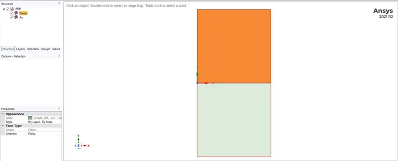
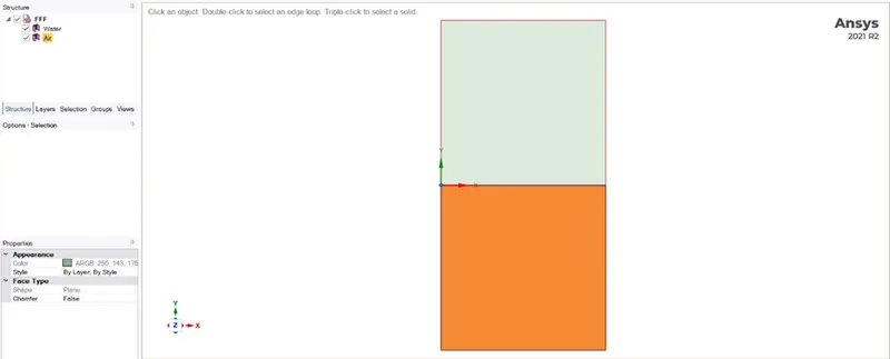
Creating 2 squares of 20mm and using ‘pull’ tool to create the surface. The upper surface will contain water and the low surface air as shown below.

Now in ‘workbench’ option select ‘share’, so that both the surfaces share a common edge

Meshing

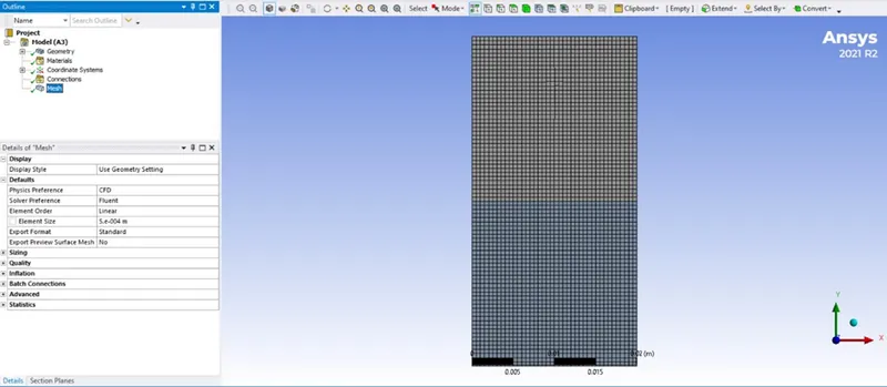
After creating the geometry, now creating a baseline mesh of 0.5mm to continue with further simulation.

Here the only difference between all the simulation is the mesh size.

For first case, Mesh size = 0.5mm

For second case, Mesh size = 0.25mm

Setting up physics

The setup will be exactly the same for the simulations. The only difference would be the mesh size.

Selecting a solver type as ‘Transient’ and enabling the gravity as shown below

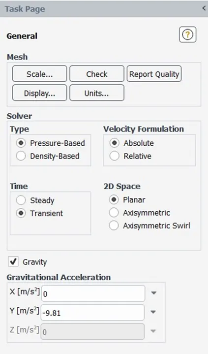
The next step would be to assign the materials i.e ‘Air’ and ‘Water’.

Under ‘Multiphase Model’ selecting ‘Volume of fluid’ as the model with ‘Implicit’ scheme as shown below

Since we will deal with only two phases in the current simulation, the number of Eulerian Phases would be assigned as 2

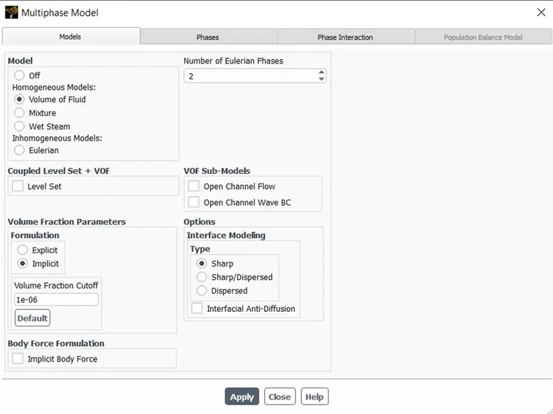
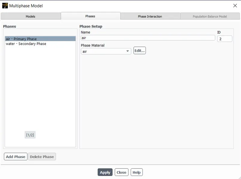
Now in Phase setup assigning the Primary phase as ‘Air’ and the Secondary Phase as ‘Water’

Before running the simulation, performing a Standard Initialization of the problem.

After this Patching process was initiated to define that at the starting of the simulation, water is in the upward potion and air is in the lower portion.

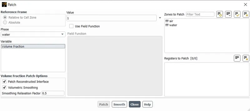
Results

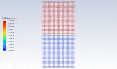
Baseline mesh

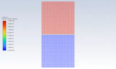
Finer mesh

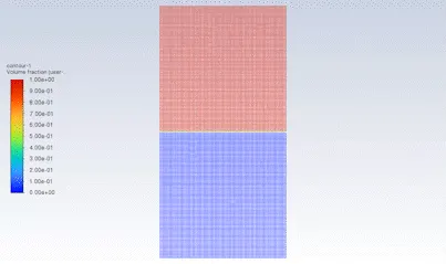
Finer mesh with user-defined material

Conclusion:-

On comparing the Baseline mesh and finer mesh it is observed that, on decreasing the mesh size, the mixing of two fluids becomes more realistic as compared to a physical case.

It can also be observed that the more we refine the mesh, the more our results gets smoother about the irregularities that take place at the interface of the two fluids.

Atwood Number

The Atwood number (A) is a dimensionless number in fluid dynamics used in the study of hydrodynamic instabilities in density stratified flows. It is a dimensionless density ratio defined as

`A = (rho_1 – rho_2)/(rho_1 + rho_2)`

Where

`rho_1` = density of heavier fluid

`rho_2` = density of lighter fluid

Atwood number is an important parameter in the study of Rayleigh-Taylor Instability. In Rayleigh-Taylor Instability, the penetration distance of heavy fluid bubbles into the light fluid is a function of acceleration time scale, `A*g*t^2`

Where g is the gravitational acceleration and t is the time

With increase in the Atwood number, the stabilization effect of initial density stratification decreases and the instability caused by the expansion-compression effect becomes more significant. The flow structures of bubbles and spikes are quite different at medium Atwood number.

Atwood number for first case in which air and water are fluids

`A = (998.2 – 1.225) / (998.2 + 1.225)`

A = 0.997

Atwood number for second case in which air and User-defined material are fluids

`A = (400 – 1.225)/(400+1.225)`

A = 0.993