Week 5 - Rayleigh Taylor Instability

AIM:

The objective of the report is to

1. Discuss some practical CFD models used to model Rayleigh Taylor model.
2. Perform air and water Rayleigh Taylor instability simulation and validate the results.
3. Perform Rayleigh Taylor instability simulation for water and user-defined material.
4. Discuss the effects of Atwood number.

THEORY:

Rayleigh Taylor instability -

Rayleigh Taylor is an instability phenomenon that occurs at the interface of two immiscible fluids of different densities. This occurs when light density fluid pushes the heavy density fluid.

Rayleigh Taylor interface instability is a complex phenomenon and the growth of instability is classified into various stages.

1. Stage 1 - The initial perturbations at the interface are extremely small such that growth of instability is assumed using linear functions. The amplitude of the perturbation grows exponentially with time.
2. Stage 2 - In this stage, the amplitude of perturbation grows non-linearly. The development of perturbations is strongly influenced by Atwood number. The Atwood number strongly influences the formation of bubbles and spikes.
3. Stage 3 - In this stage, the development of structure on the spikes and interactions among bubbles takes place. Helmholtz instability along the side of the spike can cause it to form mushroom shape.
4. Stage 4 - In the final stage, due to breakup of spike and penetration of bubbles through a slab of fluid of finite thickness, turbulent and chaotic mixing of two fluids takes place.

CFD models to validate Rayleigh Taylor instability waves -

Rayleigh Taylor instability is continuous-continuous phase interaction flow type in multi phase flow. In order to model Rayleigh Taylor instabilities, several numerical methods are introduced.

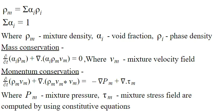
1) Single-phase model (or) Mixture model - It is the simplest method for modelling multiphase flows. In this model, the continuous phase and the discrete phase is considered as a single phase. So, in each grid cell void fraction is computed and based on the void fraction, mixture properties are defined. Eg- Mixture density, Mixture viscosity. In this model, conservation of mass equation is defined for each phase. Since, no-slip velocity is considered between discrete phase and continuum phase one momentum conservation equation is defined for the entire model.

2) Two-phase model - The two-phase model is similar to single-phase model except slip velocity is considered between the two phases. So, in two-phase model, for each phase seperate mass conservation and momentum conservation is computed. This model is also known as Euler - Euler model.

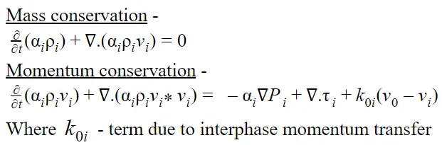
2.1) Volume of fluid method - Volume of fluid is a simpler version of full eulerian model, where all phases are treated as continuous.

3) Discrete phase method - In discrete phase model, lagrangian frame of reference is used to track particles motion and eulerian method is used to model continuous phase. Different forces like viscous, lift, drag and buoyancy force acting on the particles are taken into account.

NOTE - Generally for knudsen number << 1, Euler - euler model is preferred and for knudsen number >> 1, lagrangian particle tracking is preferred.

PROCEDURE:

In this report, simulation of Rayleigh Taylor instabilities is performed in 3 different case setup.

Case 1 - Transient state Rayleigh Taylor instabilities simulation using air and water.

Case 2 - Steady state Rayleigh Taylor instabilities simulation using air and water.

Case 3 - Transient state Rayleigh Taylor instabilities simulation using water and user defined material(density = 400 kg/m³, viscosity = 0.001 kg/m-s)

In order to perform Rayleigh Taylor instability simulation in Ansys fluent, certain steps have to be followed.

Step 1 - Geometry

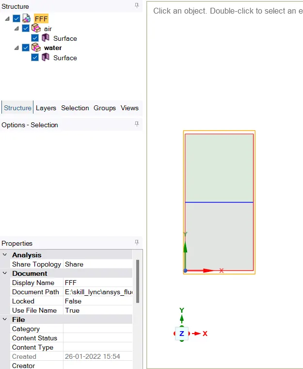
In space claim, create two components named air and water. Create rectangular shape of dimensions(20mm x 20mm). To have proper mesh connectivity between the components, create conformal mesh by sharing the topology as shown in the fig.

Step 2 - Mesh

Since, domian is rectangular in shape, quad elements are generated. Generate mesh of base size - 2.236mm, refined mesh of size 0.5mm, 0.1mm

Step 3 - Setup

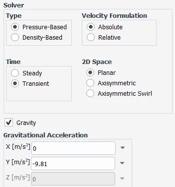
Solver type - Pressure based, Velocity formulation - Absolute, Time - tansient

In Rayleigh Taylor instability, since gravitational force is responsible for initial perturbation so include gravity in the model.

Multi Phase Model - Volume of fluid method of 2 eulerian phases are used. Implicit formulation is done.

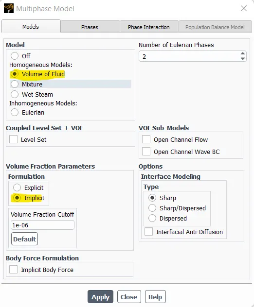
In VOF model, both phases are treated as coninumm phases. In this model primary phase is air and secondary phase is water.

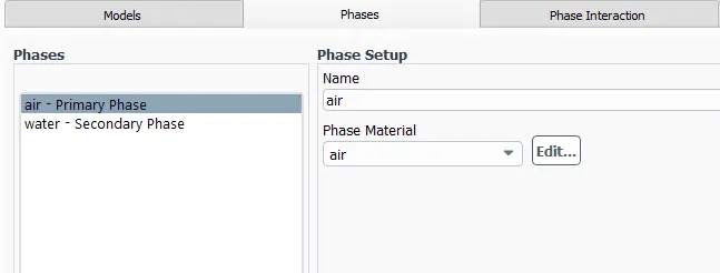
Boundary conditions - Wall boundary conditions are imposed.

P-V Coupling scheme - Simple

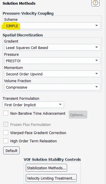
Initialize the model with standard method.

In multi phase flows, it is important to patch the geometry. In this report, patch the geometry with phases so that void fraction contours are plotted accurately.

Perform calculation with fixed time step size dt = 0.005, no.of steps = 1500

Results -

Air and Water material

Transient-state:

The following plots shows the volume fraction contours of air and water. The transient state analysis is done for 3 different mesh size - 2.236mm, 0.5mm, 0.1mm. Initially at t = 0sec, air is at bottom and water is at top. Due to density difference, at end state, the heavier fluid water settles at bottom and lighter fluid air settles above the water.

From the above plots, compared to 0.5mm, 0.1mm mesh size for 2.236mm mesh size, the initial perturbations and growth in the instabilities are not clearly visible. The 0.1mm mesh is much-refined(Fine)mesh compared to 0.5mm but the computational time is more.

Steady-state:

The above plot shows the Rayleigh Taylor instabilities of mesh size 0.5mm computed by using steady state analyis. So, from the contours, it is observed that the initial perturbations and growth in instabilities are not visualized clearly in steady-state analysis compared to transient setup. Since, steady state analysis captures only final effects, it is preferred to perform instability analysis like Rayleigh Taylor, kelvin helmholtz by using transient case.

Water and user-defined material:

Atwood number:

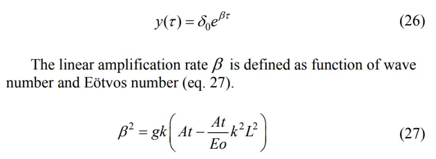
It is discussed in the above sections that initial growth linear of perturbations is exponential with time and depends on the atwood number (At).

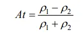, where ρ1 is higher density fluid and ρ2 is lighter density fluid.

Higher the value of Atwood number greater will be the growth of initial disturbances.

1. Air and Water, At = (998.2 - 1.225)/(998.2 + 1.225) = 0.997
2. Water and user difined material, At = (998.2 - 400)/(998.2 + 400) = 0.427

Since, Atwood number for water and user defined material is less compared to Air and water medium, initillay at t >0sec the rayleigh taylor instabilities is small for water and user defined material.

CONCLUSION:

The different CFD models used to compute multiphase flows and the theory of Rayleigh Taylor instabilities are discussed. It is concluded that transient state analysis capture rayleigh taylor instabilities accurately compared to steady-state analysis. The Atwood number of air and water medium is more compared to Atwood number of water and user-defined material, so the amplitude of initial perturbations are high for air and water material compared to water and user-defined material.