Week 5: Prandtl Meyer Shock problem

Aim:

• Simulate the supersonic and subsonic flow through a duct having a sharp edge.
• Study the formation of shock waves and observe the effect of SGS parameter on shock location and cell count.

What is a Shock wave?

A shock wave or shock is a type of propagating disturbance that moves faster than the local speed of sound in the medium. Like an ordinary wave, a shock wave carries energy and can propagate through a medium but is characterized by an abrupt, nearly discontinuous, change in pressure, temperature, and density of the medium. The shock wave is a strong pressure wave in any medium either in air or water. It is created by explosions, lightning, supersonic aircraft, and other phenomena that create violent changes in pressure.

In supersonic flows, additional increased expansion may be achieved through an expansion fan also known as a Prandtl Meyer expansion fan. The accompanying expansion wave may approach and eventually collide and recombine with the shock wave, creating a process of destructive interference. When a shock wave passes through matter, energy is preserved but entropy increases. The sonic boom associated with the passage of a supersonic aircraft is a type of sound wave produced by constructive interference.

Shock flow boundary conditions:

Boundary conditions are generally three types. They are the Dirichlet boundary condition, Neumann boundary condition, and Robin boundary condition. When using a Dirichlet boundary condition, the value of the function is prescribed at the boundary. In the Neumann boundary condition, the value of the normal derivative of a function is specified. In Robin boundary condition is the combination of both the above boundary conditions, specified at both ends.

Here the variables(pressure, temperature, Mach no., and velocity) are not available at the beginning. So nothing is specified at a supersonic outlet and all variables are extrapolated from the domain interior. Only the normal derivative of variables are specified as zero. So, Neumann boundary conditions are used in supersonic outlets.

Prandtl Meyer expansion fan or expansion fan:

A supersonic expansion fan, technically known as Prandtl–Meyer expansion fan, a 2D simple wave, is a centered expansion process that occurs when a supersonic flow turns around a convex corner. The fan consists of an infinite number of Mach waves, diverging from a sharp corner. When a flow turns around a smooth and circular corner, these waves can be extended backward to meet at a point. The below image shows the expansion fan setting diverging lines from the corner.

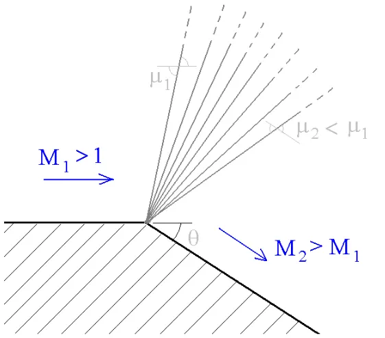
Each wave in the expansion fan turns the flow in small steps. It is physically impossible for the flow to turn through a single shock wave because this would violate the 2nd law of thermodynamics. Across the expansion fan, the flow accelerates (velocity increases) and the Mach number increases, while the static pressure, temperature, and density decrease. Since the process is isentropic, the stagnation properties (total pressure and total temperature) remain constant across the fan.

Procedure:

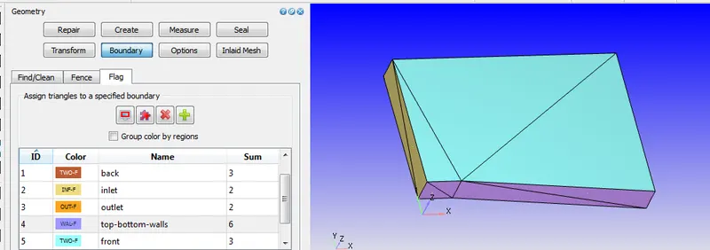
1. Select the faces of the body give the boundary names as shown in the below figure. After that click on the normal toggle to check that all normals are pointed towards the flow.

2. case setup:

2.1 Select time-based in the application type. And click on materials and set them to default.

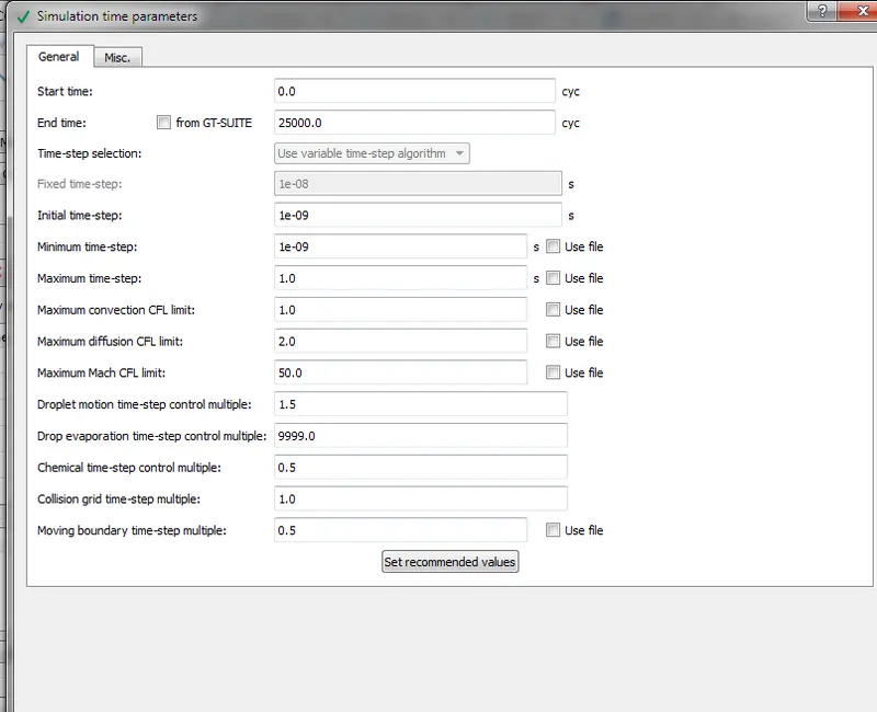
2.2 Simulation parameters: Select steady-state solver in run parameters and coming to solver parameters set Navier stokes solver type to density-based.

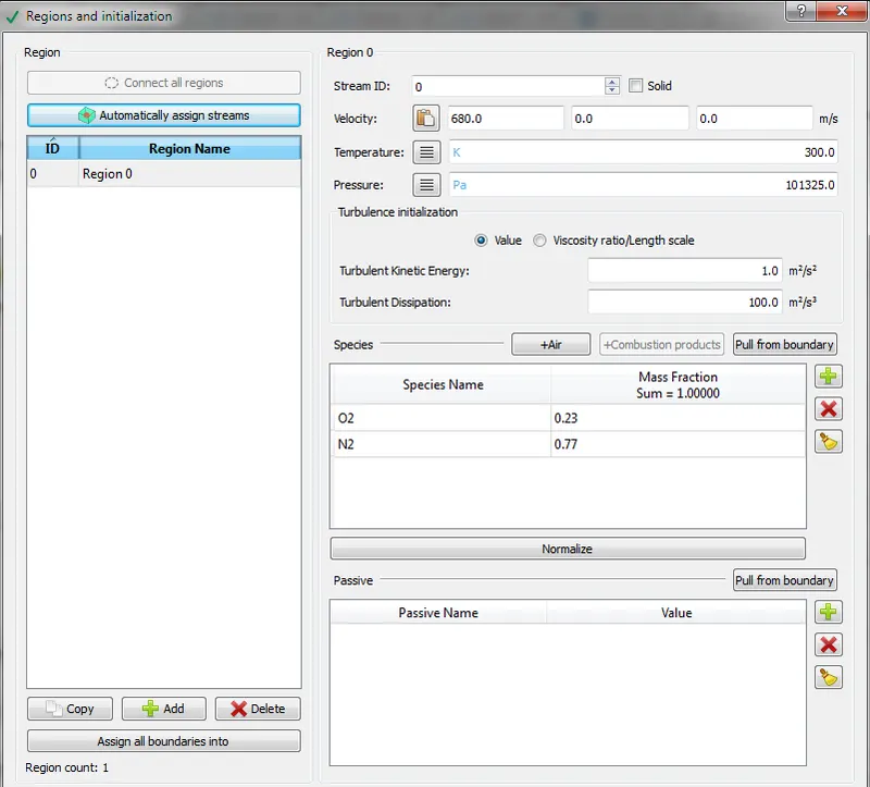
2.3 Initial conditions and events:

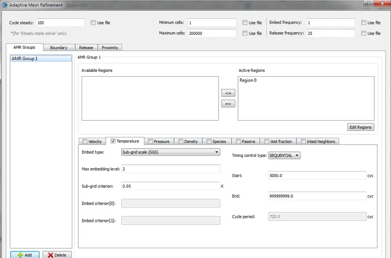
2. 4 Grid control: The base grid size is equal to 0.8. Select adaptive mesh refinement and enter the values. Mention SGS parameter as 0.05.

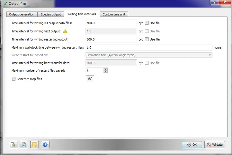
2.5 Output/ post-processing:

2.6 Boundary conditions:

The front and back faces have boundary types as TWO-D. And coming to inflow, outflow, and top-bottom walls boundary types as inflow, outflow, and walls. Here the velocity is 650 then it is a supersonic flow and the velocity value is 100 then it is a subsonic flow.

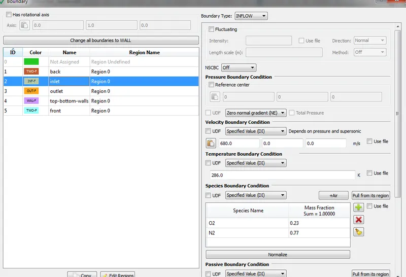
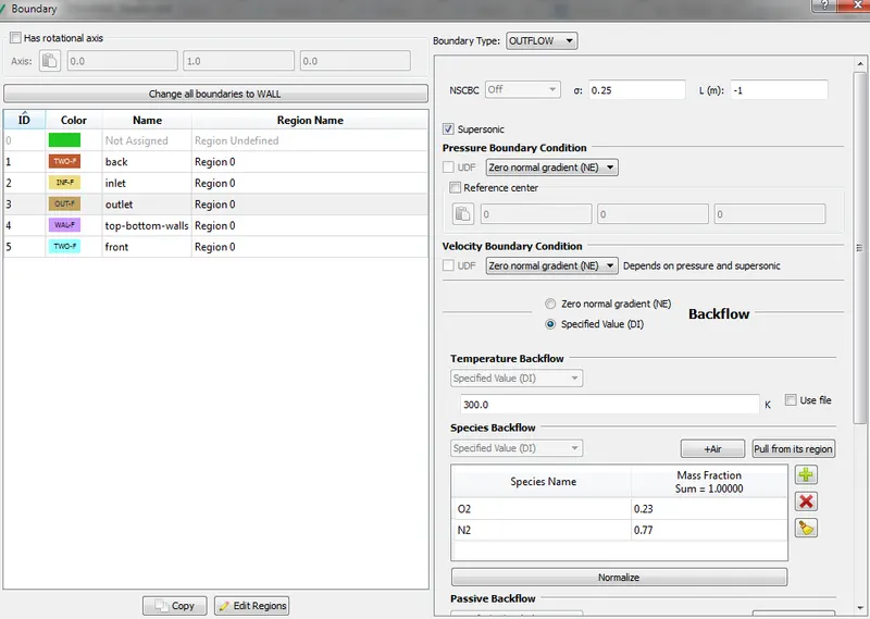
Here 3 cases are set and those are for subsonic and supersonic flow and for low and high SGS parameters.

3. Now export all input files: Click on files > Export > Export input files > choose the path and select all files and press ok.

4. Run the simulation and post-convert the files: Copy and paste the mpiexec.exe file and converge.exe file to the folder in which the input files are exported to run the simulation in Cygwin. Copy the post_convert_30_msmpi_64.exe file and paste it into the output folder. Now open Cygwin and go to the output folder and type mpiexec.exe -n 4 post_convert_30_msmpi_64.exe > enter the case name(as case1) > select file type as Paraview VTK in-line binary format > type all for files and cell variables and click enter (or) we can convert those files in converge studio.

5. Post-processing the files:

To post-process the files lanch paraview and open the file location as case1 which is saved in output > case1 .. vtm (this is a group file which is formed during post-converting the files) > click on apply > create a slice along the z-axis.

Results:

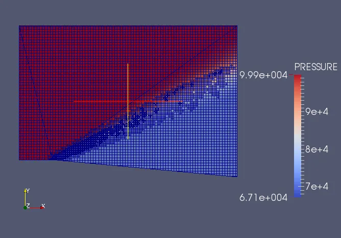
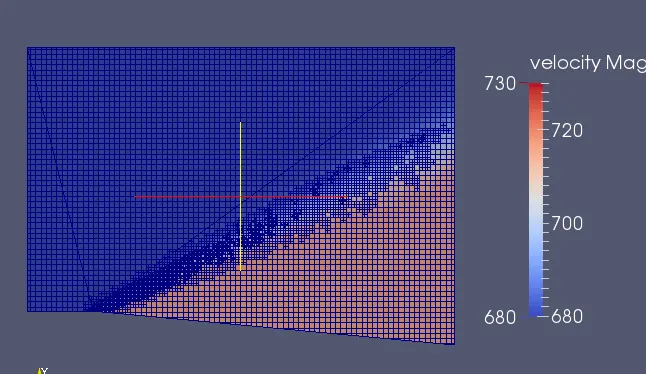
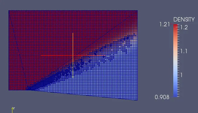
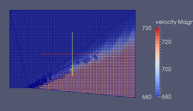
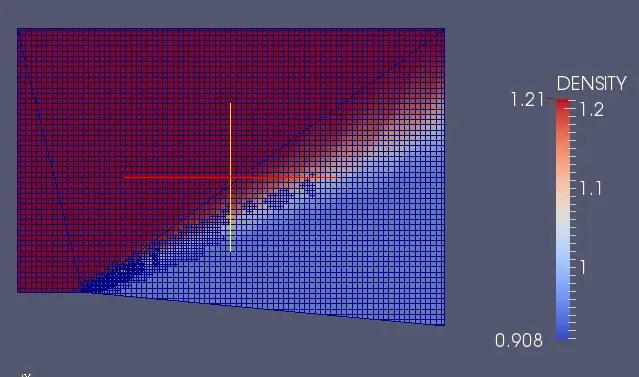
Case 1: Countors for Supersonic flow

Plots:

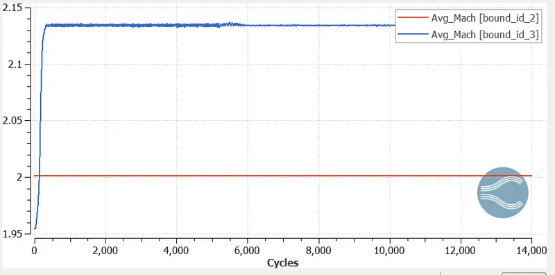
Mach number:

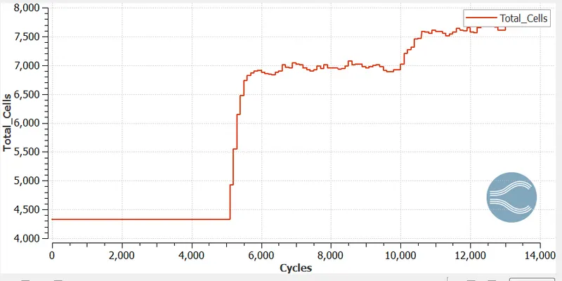
Total cells:

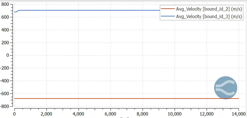
velocity:

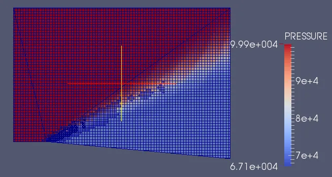
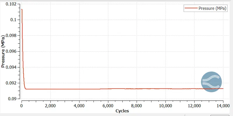
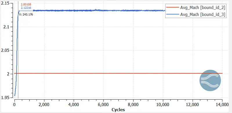
Case 2: Countors for Supersonic flow with low SGS parameter(0.1)

Plots:

Pressure:

Mach number:

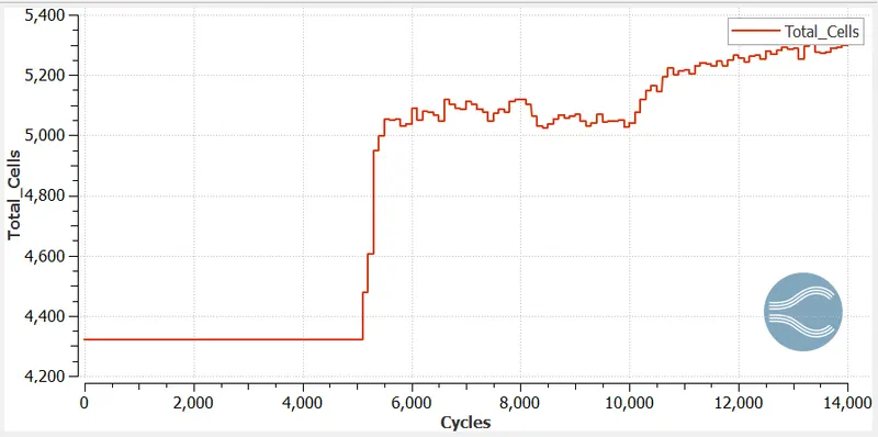
Total cells:

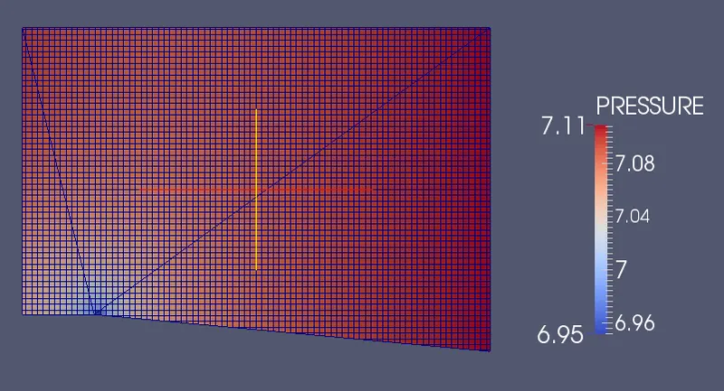
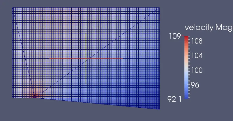
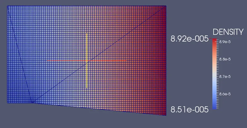
Case 3: Countors for Subsonic flow(velocity=100, SGS = 0.05)

Plots:

Pressure:

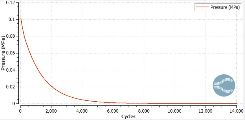
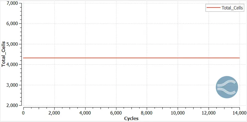
Total cells:

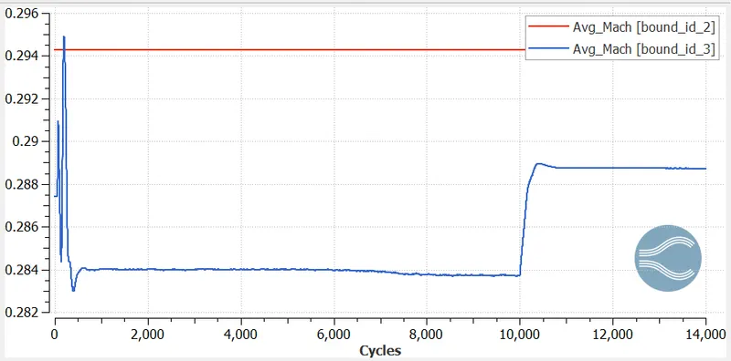
Mach number:

Animation link:

Case1: https://youtu.be/YG0oyuFnDxw

Case2: https://youtu.be/ZFdjCvviUvY

Case3: https://youtu.be/0haNu2YCFRQ

Effect on SGS parameter on shock location and total cell count:

• From the above results, the SGS parameter decreases the total cell count increases and there is more formation of cells around the shock wave.
• For a high SGS parameter, the mesh refinement area is very small like in case-2.

Conclusion:

• In supersonic flow, the Prandtl-Meyer expansion fan is clearly visible and the mesh refinement is also visible in the shock region.
• Whereas in the subsonic flow, the Prandtl-Meyer expansion fan is not visible at all and the mesh refinement is also not visible. This is due to there is no shock waves(sudden change in pressure, temperature, velocity, and density).
• As the SGS parameter decreases, the total cell count increases and the mesh refinement area spread from the sharp edge to the outlet boundary. If the SGS parameter increases, the mesh refinement area is very small and it doesn't spread to the outer boundary.