Week 5: Prandtl Meyer Shock problem

1. Title – Steady state simulation of flow over a throttle body.

2. Objective –

• To create the CAD model in which shock wave can be created, in converge Software.
• To set up the case with proper grid size, material and boundary conditions.
• To solve the case using Cygwin terminal and convert the result for Paraview software.
• To import output files in Paraview and generate required contours and plots.

3. Theory –

Shock wave is a propagating disturbance, produced by supersonic aircraft, lightning, explosion or other phenomenon, which creates violent change in pressure or we can define shock wave, which moves faster than sound in the medium. Shock wave propagate in different manner than ordinary sound wave, particularly, shock waves travel faster than sound, and their speed increases as the amplitude is raised, but the intensity of a shock wave also decreases faster than does that of a sound wave, because some of the energy of the shock wave is expended to heat the medium in which it travels.

According to doppler effect, the observed frequency increases when the source approaches the speed of sound. What if source moves equal to or more than speed of sound, well according to doppler effect it will make observer infinite. At the speed of sound, this result means that in front of the source, each successive wave interferes with the previous one because the source moves forward at the speed of sound. The observer gets them all at the same instant, so the frequency is infinite. If the source exceeds the speed of sound, no sound is received by the observer until the source has passed, so that the sounds from the approaching source are mixed with those from it when receding. This mixing is shock wave.

Boundary conditions for the wave equation describe the behaviour of solutions at certain points in space. Different types of boundary conditions can be imposed on the boundary of the domain. The selection of type of boundary conditions depends on the domain, we are working. Boundary conditions has many types like Dirichlet Boundary condition, Neumann boundary conditions, Cauchy boundary condition, Robin boundary conditions etc. generally Dirichlet Boundary condition and Neumann boundary conditions are used for shock wave. In this simulation we will use Dirichlet Boundary condition, which will specify velocity and temperature at the boundary.

Sub grid scale – it is a feature which refines grid based on the particular parameter- temperature, velocity, pressure, density etc. it refines mesh automatically by applying sub grid criteria like sub grid criterion 4m/s, it will refine mesh at area where curvature of velocity is above 4m/s. embedded layers can be introduced as well. The embedded grid size is given by following formula –

Grid size = base grid/2^embedded level

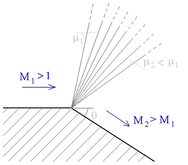
Prandtl-Meyer expansion fan is a centred expansion process, which turns a supersonic flow around a convex corner. The fan consists of infinite number of Mach waves, diverging from a sharp corner. In case of a smooth corner, these waves can be extended backwards to meet at a point. Across the expansion fan, the flow accelerates means velocity increases and the Mach number increases, while the static pressure, temperature and density decrease.

4. Procedure –

In this simulation will simulate shock flow. We made CAD model which mimics Prandtl-Meyer expansion fan. Through this expansion will simulate shock wave for three different sub grid criterions. For this simulation following procedure was followed -

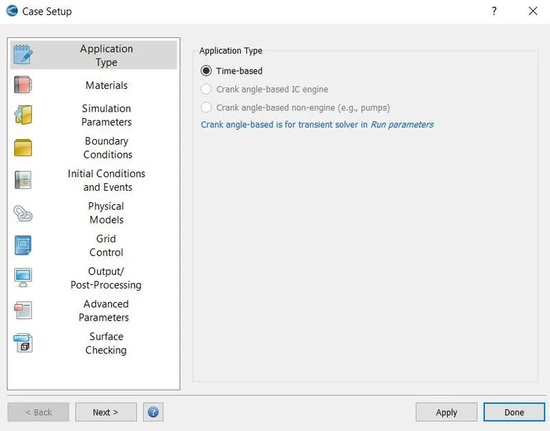
1. Started with the choosing application type, we chose time based this simulating does not related to IC engine or other mechanism with has crack angle parameter.

Case setup - Application type

2. Air was chosen as fluid with enabled reaction mechanism.

Material selection -

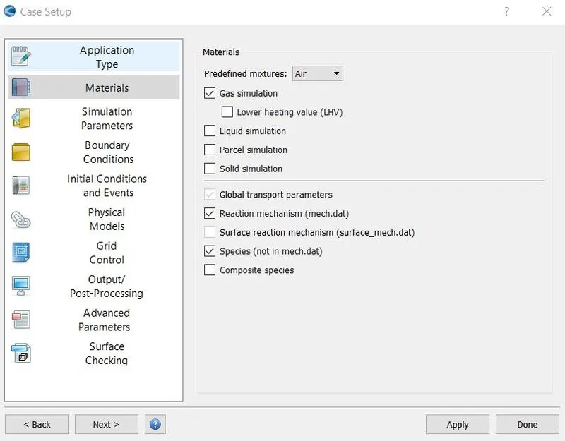
3. Parameters of gas simulation, global transport parameters were kept same.

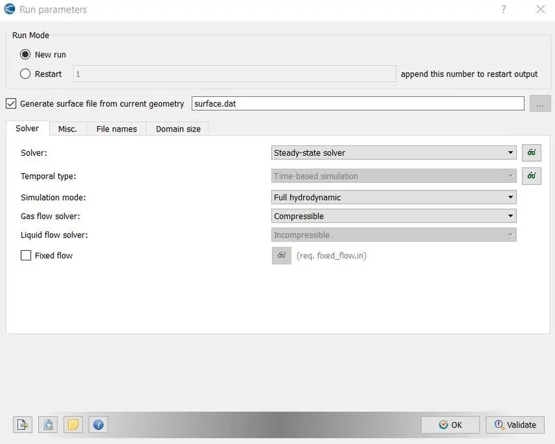
4. In run parameters steady state solver was chosen, because in this simulation fluid is continuous and it gets steady state after some time. Simulation mode is chosen as Full hydrodynamic, because we want to simulate with effect of fluid also, if someone want to see quality of mesh and its effect only, he can go with no hydrodynamic option. Air is compressible so we went with that option.

Run parameters -

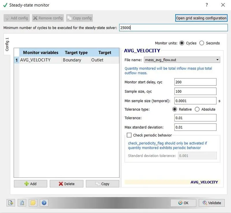
5. If someone want to monitor parameters, he can enable option steady state, we selected average velocity as parameter.

Steady state monitor -

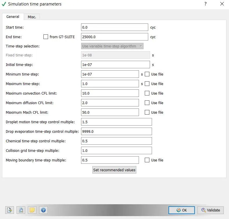
6. Simulation time parameter is important parameter which decides simulation stability, number of time steps which is iterations, minimum and maximum time step etc. we went with 25000 cycles with stating at 0 second, minimum time step and initial step 1e-07, maximum time step of 1 second. These parameters will affect simulation time. Maximum convection CFL limit was reduced from 10 to 1 to get stable solutions. CFL limit decides the stability of simulation, if it is high than solution will get fluctuations.

7. In solver parameters pressure-based solver was selected and 1 was set as maximum convection CFD limit for final stage.

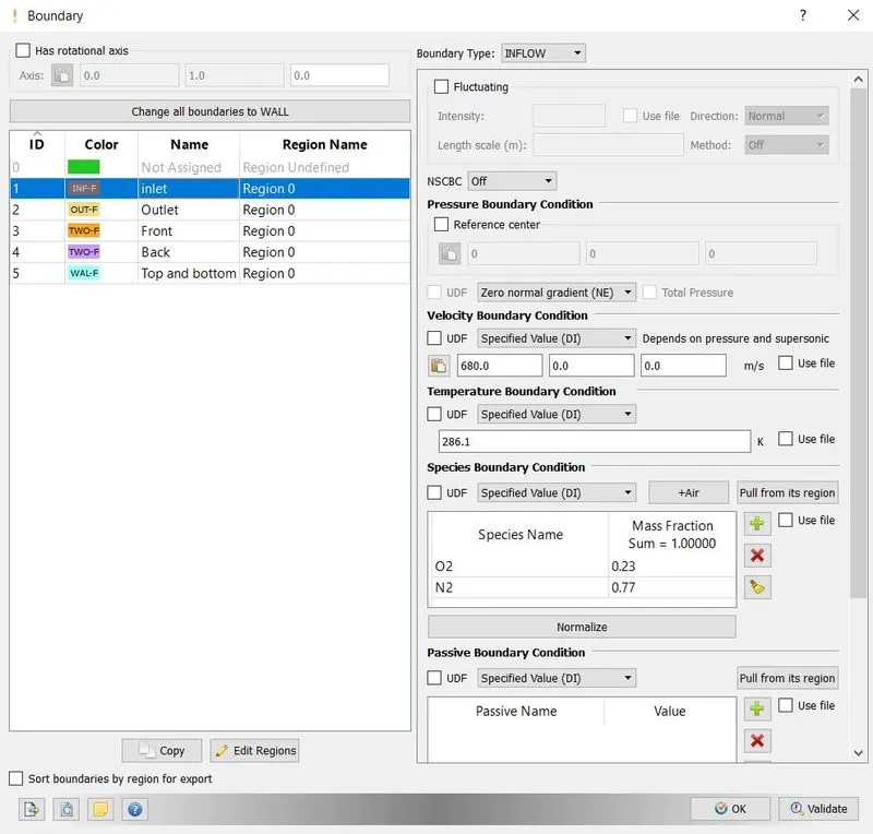
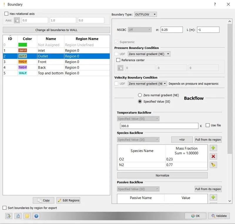
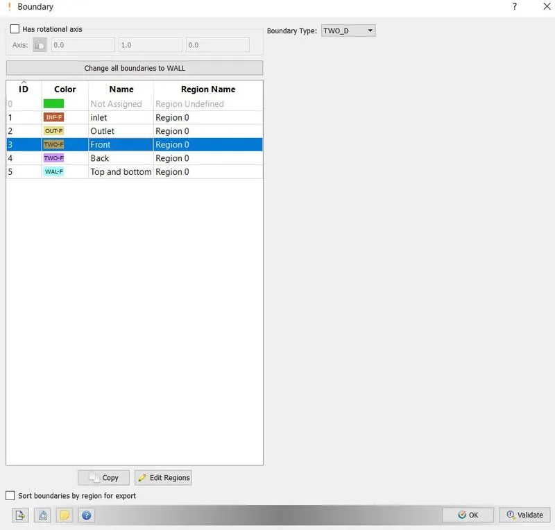
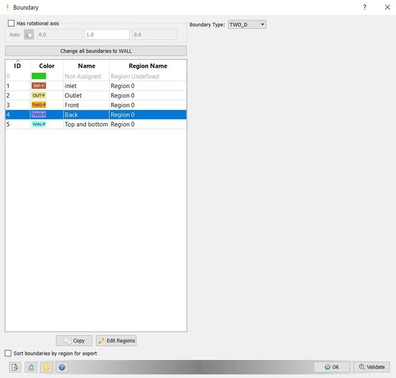
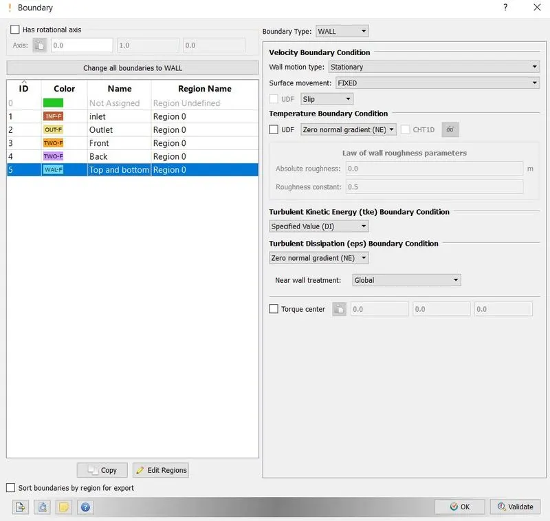
8. In boundary conditions inlet was set with inflow and velocity 680m/s, temperature 286.1K were given. At outlet outflow boundary was set and pressure and velocity were fixed with zero normal gradient. Front and back boundaries set with 2D boundary and top and wall boundary was set with slip.

Boundary Conditions -

Inlet -

Outlet -

Front and Back -

Top and bottom -

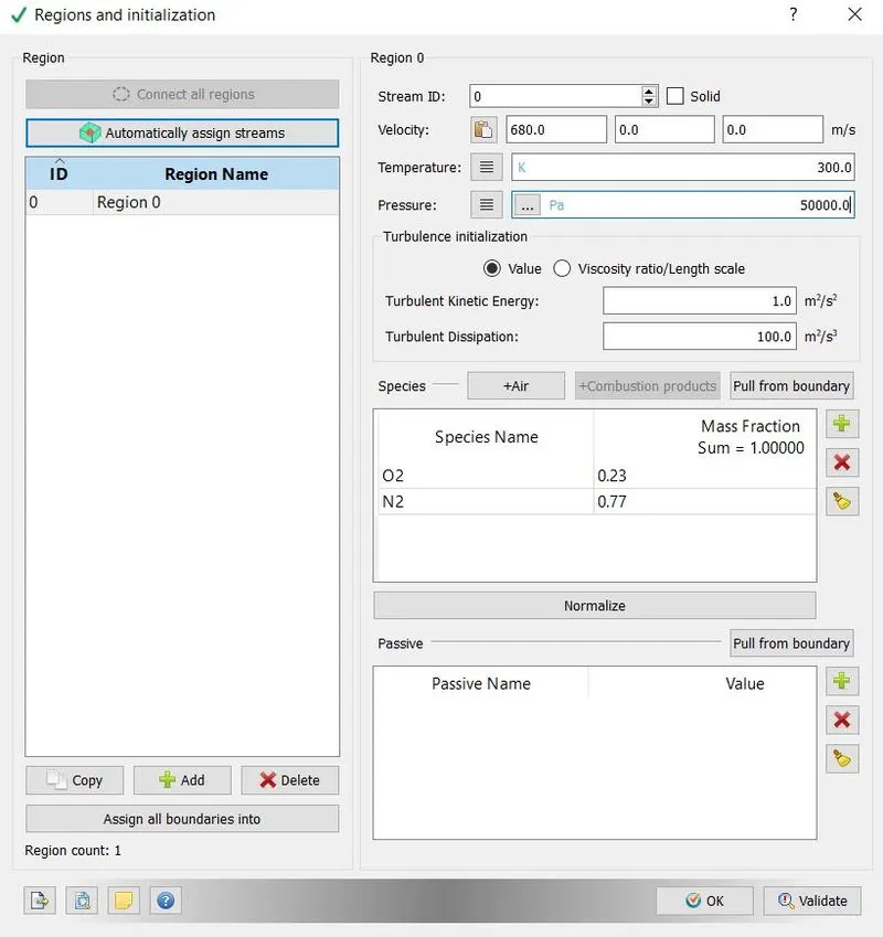
9. Region was created which helps to initialize the solution. In boundary conditions this region was selected for all boundaries as region type. We passed the value of velocity 680m/s, pressure 50000 and temperature 300K in regions parameter.

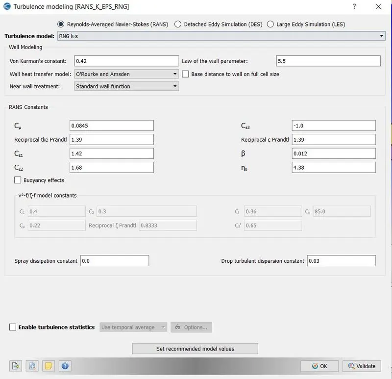
10. Reynolds averaged Navier-Stokes was selected as turbulence model with default parameters.

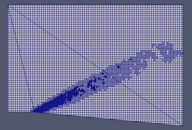
11. In base grid option the size of mesh was selected with option adaptive mesh refinement. This option allows us to refine mesh at particular area with the values of any parameters like temperature, velocity, density etc. in this simulation we wanted to refine mesh according to temperature values. In adaptive mesh refinement menu temperature option enabled with embedding level of 2 and sub-grid criterion 0.0,0.05,0.04(three different cases). Values of starting and ending cycle were also given as shown in the image. Embedded level 2 refines the according to above written formula (in theory).

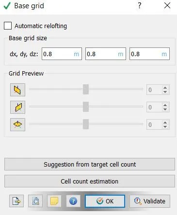
Base grid = 0.8m

At level 1 embedding = 0.8/2^1 = 0.4m

At level 2 embedding = 0.8/2^2 = 0.2m

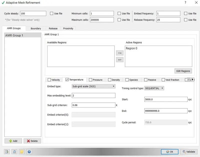
So, 0.2m is the lowest mesh size, which is used in this simulation. Sub grid criteria decides, when to refine mesh like we used sub grid criteria 0.05K means mesh will be automatically refines when curvature of temperature goes above 0.05K.

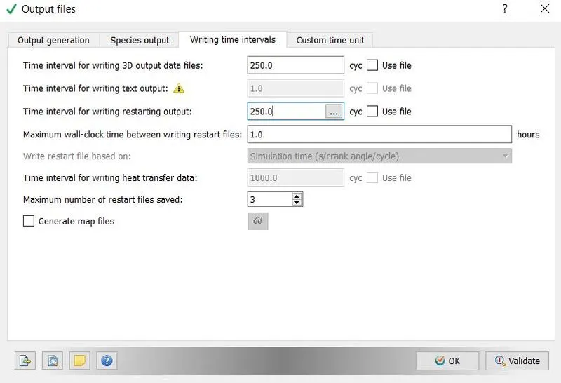
12. Post variable selection was kept unchanged because it has necessary variables selected as defaults. Output files option defines the time interval for writing output data, restarting output etc. we gave 250 as time interval to write data file and time interval for restarting, because we wated 100 output files. We were simulating for 25000 cycle and want an output file after 250 cycle so it is obvious that we will get 100 output files. Restart files allows you to restart simulation from particular time step.

5. Results –

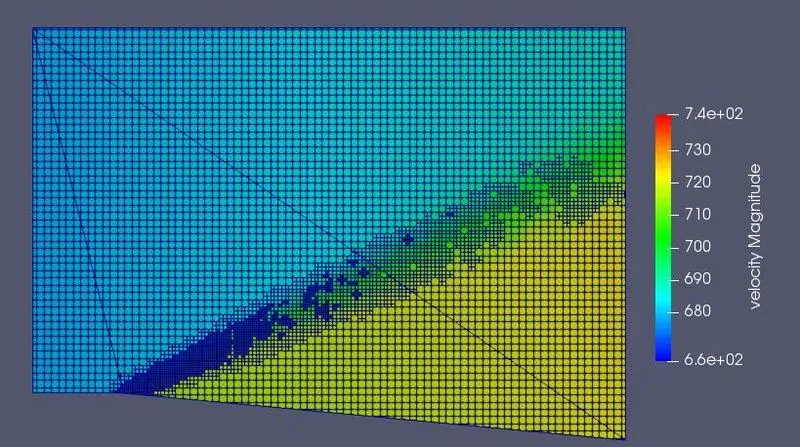
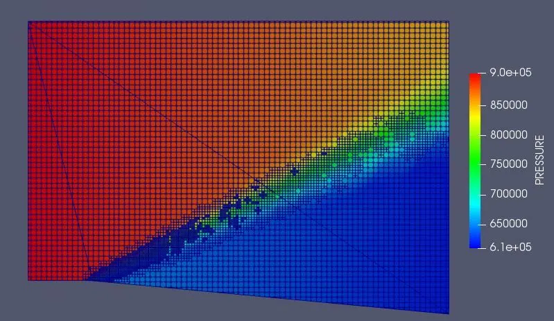
Case 1 SGC -0.05

Mesh -

Velocity -

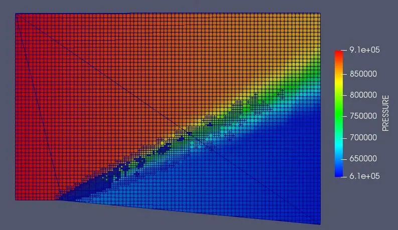
Pressure -

Velocity animation - https://drive.google.com/file/d/185brhaRMRP4kmSoLGHMyn_8SUu40MEy0/view?usp=sharing

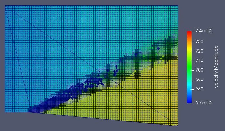
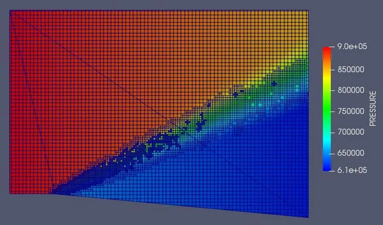
Case 2 SGC -0.04

Mesh -

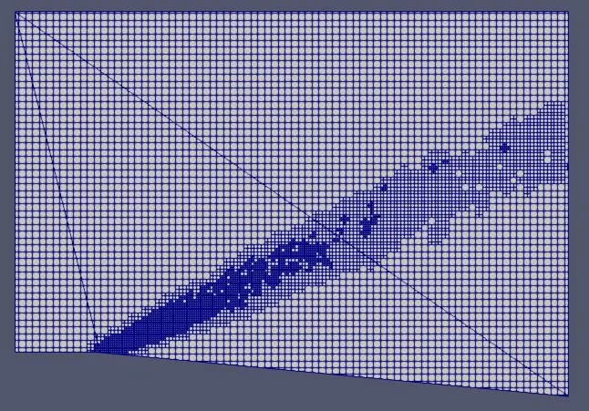
Velocity -

Pressure -

Velocity animation - https://drive.google.com/file/d/1lAN1TJ95WupJxzdx5JmQGWrivbTPR_Zf/view?usp=sharing

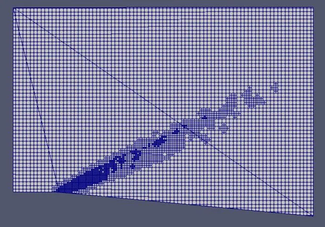
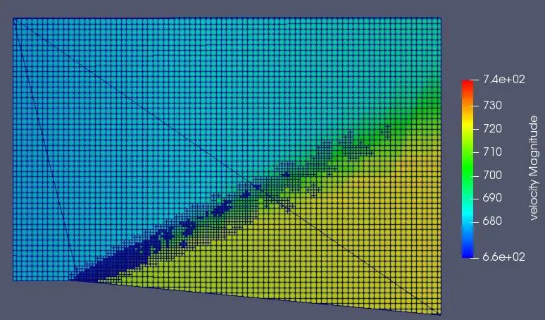
Case 3 SGC -0.06

Mesh -

Velocity -

Pressure -

Velocity animation - https://drive.google.com/file/d/1mGKmMzp-bEmtz_Xez6sCp7lerKJGFxaQ/view?usp=sharing

Amination of velocity has generated to get insights of mesh refinement and wave propagation. We can observe from animation that sub grid scale is clearly affecting the shock wave visibility. Sudden expansion in surface greatly affects the pressure (decreases) and it results into shock wave generation.

6. Conclusion –

The main aim of this simulation was to generate shock wave and study the effect of sub-grid scale on shock wave. We show how an abrupt surface leads to generate shock wave. The results of this simulation, validates the theory of shock wave generation. We got maximum velocity of wave 740m/s and minimum velocity 660m/s, which is due to high pressure.