Week 5: Prandtl Meyer Shock problem
JORGE LOZANO
Advanced CFD for IC Engine Applications using Converge
Prandtl Meyer Shock problem
Objective
- Shock flow boundary conditions
Do a literature search on what BC's are typically used for shock flow problems
- What is a shock wave?
In your own words, describe the physics behind shock waves
- Effect of SGS parameter on shock location
In the Prandtl Meyer shock problem, look at the effect of SGS temperature value on cell count and the shock location
It is expected to show the mesh generation using PARAVIEW.
Also create an animation and upload it on You tube and provide the You tube link for an animaion in your report.
Documentation
Shock wave
Shock wave, strong pressure wave in any elastic medium such as air, water, or a solid substance, produced by supersonic aircraft, explosions, lightning, or other phenomena that create violent changes in pressure. Shock waves differ from sound waves in that the wave front, in which compression takes place, is a region of sudden and violent change in stress, density, and temperature. Because of this, shock waves propagate in a manner different from that of ordinary acoustic waves. Shock waves travel faster than sound, and their speed increases as the amplitude is raised; but the intensity of a shock wave also decreases faster than does that of a sound wave, because some of the energy of the shock wave is expended to heat the medium in which it travels. The amplitude of a strong shock wave, as created in air by an explosion, decreases almost as the inverse square of the distance until the wave has become so weak that it obeys the laws of acoustic waves. Shock waves alter the mechanical, electrical, and thermal properties of solids and, thus, can be used to study the equation of state (a relation between pressure, temperature, and volume) of any material.
Sub-grid Scale (SGS)
The simulation of turbulent flow has been a considerable challenge for many decades. There are three main approaches to compute turbulence: 1) the Reynolds averaged Navier-Stokes (RANS) approach, in which all turbulence scales are modeled; 2) the Direct Numerical Simulations (DNS) approach, in which all scales are resolved; 3) the Large Eddy Simulation (LES) approach, in which large scales are computed, while the small scales are modeled.
Although the RANS approach has achieved wide-spread success in engineering design, some applications call for LES, e.g., flow at high-angles of attack. The spatial filtering of a non-linear PDE results in a SGS term, which needs to be modeled based on the resolved field. The earliest SGS model was the Smagorinsky model, which relates the SGS stress with the rate-of-strain tensor. The purpose of the SGS model is to dissipate energy at a rate that is physically correct. Later an improved version called the dynamic Smagorinsky model was developed by Germano et al. and demonstrated much better results.
Pre-processor
Geometry & Case Setup
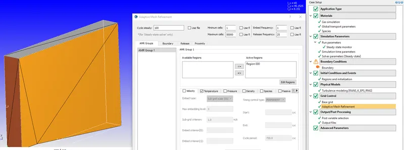
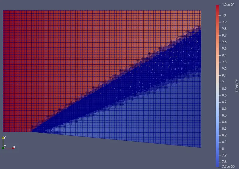
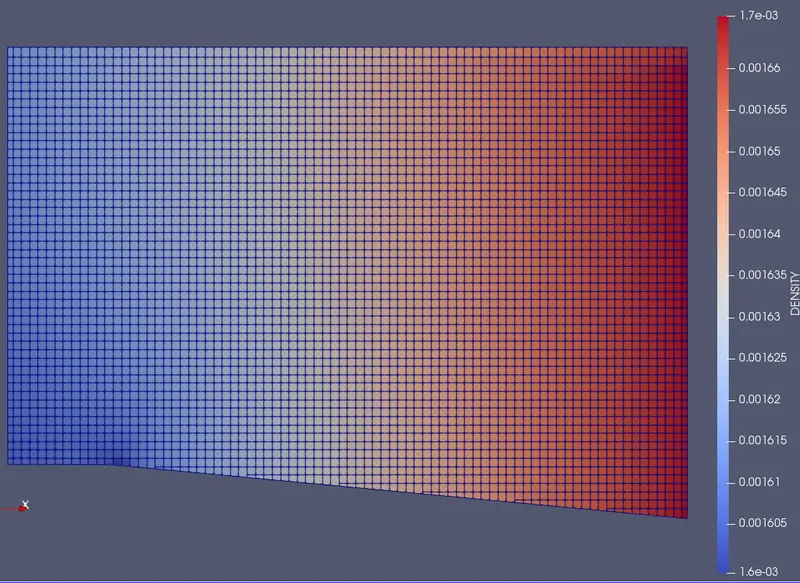
In this challenge the cases are simulated to obtain the results and effects of having a supersonic and subsonic flow system, where in the three cases are using a SGS mesh generation in the variation of temperature gradient of 0.05, 0.005 and 0.05 Kelvin, and 680, 680 and 100 m/s as velocity. A RANS turbulent modelling is being used to determine the average fluctuations of velocity, having a refinement in a visual diagonal region.
Postprocessing
Steady state cases
Paraview
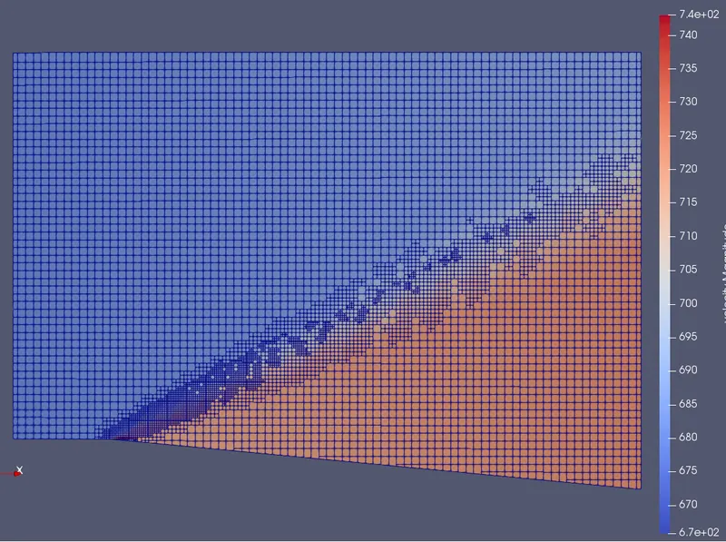
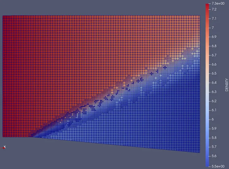
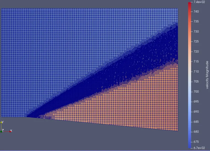
The following images show the contours asked for, for analyzing and seeing the results obtained.
Velocity Mesh end case 1
Density Mesh end case 1
Velocity Mesh end case 2
Density Mesh end case 2
Velocity Mesh end case 3
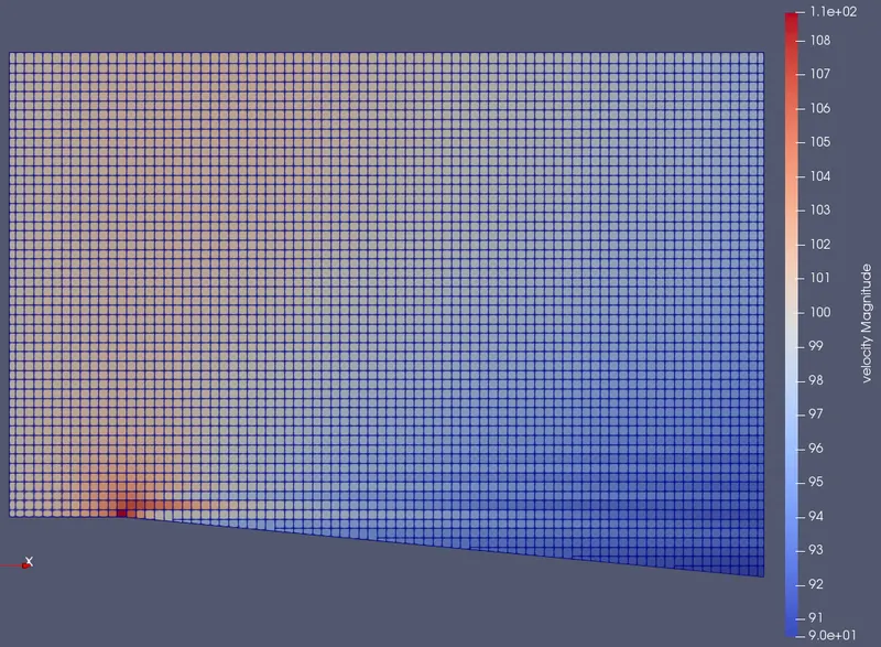
Density Mesh end case 3
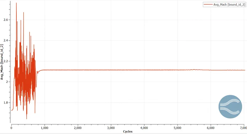
Converge plots at a specific time
Mach number case 1
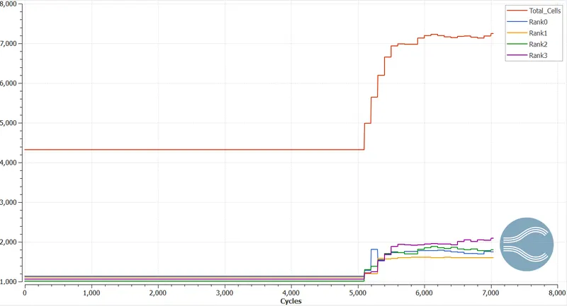
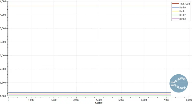
Cell count per processor case 1
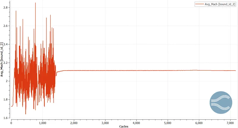
Mach number case 2
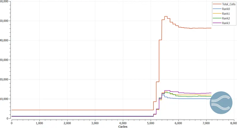
Cell count per processor case 2
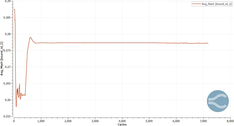
Mach number case 3
Cell count per processor case 3
Conclusion
- Shock flow boundary conditions
INLET Pressure boundary condition
Zero normal gradient (NE): Neumann - To run the simulation without pressure transfer between the boundary and the fluid, select Zero normal gradient (NE). You can use the NE Pressure boundary condition with only the following Velocity boundary conditions:
Dirichlet (DI)
Mass flow (MA)
Pump (PU)
OUTLET Pressure boundary condition
Zero normal gradient (NE): Neumann - To run the simulation without pressure transfer between the boundary and the fluid, select Zero normal gradient (NE). You can use the NE Pressure boundary condition with only the NE Velocity boundary condition. To use this option with the NE Velocity condition, the Supersonic box must be checked.
Neumann and Dirichlet boundary conditions [5]
- What is a shock wave?
Shock waves are steep fronts that propagate in the compressible fluids in which convection dominates diffusion. They are fundamental in nature, especially in high-speed fluid flows. Examples include transonic and/or supersonic shocks formed by supersonic flows impinging onto solid wedges, transonic shocks around supersonic or near sonic flying bodies, bow shocks created by solar winds in space, blast waves by explosions, and other shocks by various natural processes. When a shock hits an obstacle, or a flying body meets a shock, shock reflection/diffraction phenomena occur. Many of such shock reflection/diffraction problems can be formulated as free boundary problems involving nonlinear partial differential equations (PDEs) of mixed elliptic-hyperbolic type. The understanding of these shock reflection/diffraction phenomena requires a complete mathematical solution of the corresponding free boundary problems for nonlinear mixed PDEs.[3]
- Effect of SGS parameter on shock location
When the beginning of the SGS mesh refinement happens, the cell numbers increases and the variables converge at a more accurate level, due to the closeness of the cells, having the second case where the variation is more sensitive a wider refinement region and a more precise system, where in the third case it does not have any refinement because density and temperature properties aren’t being affected by the subsonic system.
VIDEO CASE 1
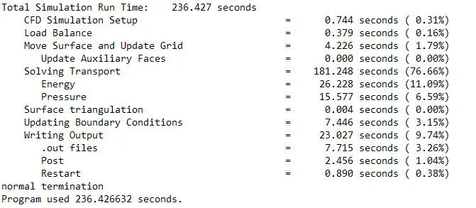
TIME ANALYSIS CASE 1
VIDEO CASE 2
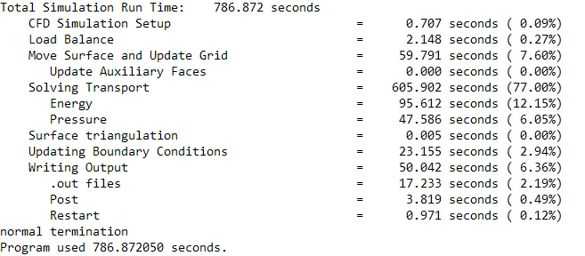
TIME ANALYSIS CASE 2
VIDEO CASE 3
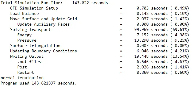
TIME ANALYSIS CASE 3
References
- https://www.britannica.com/science/science
- http://cfd-zjw.blogspot.com/2017/11/sub-grid-scale-sgs-stress-models-in.html
- https://www.maths.ox.ac.uk/system/files/attachments/OxPDE%2015.06.pdf
- https://reader.elsevier.com/reader/sd/pii/S209526861400192X?token=7680F8ED15313EC82B5DD5CD92FFD94999BDEABBD31F9C4FFDFDE7602ED97B5593D89D76C45EE890B917D41012E55D29&originRegion=us-east-1&originCreation=20210405205738
- http://www.bakker.org/dartmouth06/engs150/06-bound.pdf