Week 5: Prandtl Meyer Shock problem

Literature Review on Boundary Conditions:

1. Dirichlet boundary condition
In Dirichlet boundary condition, the value of function is specified at the boundary.This boundary condition is generally used while solving linear problems.

2. Neumann boundary condition
In Neumann boundary condition, the value of normal derivative of a function is specified.It is imposed on an ordinary or a partial differential equation and specifies the values that the derivative of a solution is assigned to the boundary of the domain. This boundary condition is generally used in non-linear problems

3. Robin boundary condition:
It is the combination of both the above boundary conditions, specified at both the ends.It is a weighted combination of the Dirichlet boundary and the Neumann boundary condition in all the parts of the boundary.

4. Mixed boundary conditions
One one end there is dirichlet boundary condition and on the other end there is Robin boundary condition.The mixed boundary condition refers to the cases in which Dirichlet boundary conditions are assigned in one end of the boundary while Neumann boundary conditions is assigned to the other end.

Why is Neumann Boundary condition used for supersonic Outflow?
Because the values of the all the variables (pressure, velocity, temperature, Mach no) are not available before solving the problem. So nothing is specified at a supersonic outlet and all variables are extrapolated from the domain interior. Only the Normal derivative (Normal with respect to the outlet boundary) of variables are specified as 0 (or Zero Gradient). However, if any pressure value or velocity is specified at the outlet the solution will not converge and become unstable.

In Neumann boundary condition, the value of the gradient of the dependent variable (flux) is provided along the boundary of the domain. For example, a perfect insulator would have no flux while an electrical component may be dissipating at a known power.
Pressure gradient at the outlet. It proves as a driving factor for the fluid flow.. In Neumann boundary conditions, the states through the simulations are devised as differentials of the initially defined flow characteristics and are thus extrapolated. In supersonic flow, characterized by abrupt changes in state parameters, a steady value of parameters post flow are a rare case and thus extrapolated Neumann boundary conditions are employed.

Shock wave:

Shock wave is a propagating disturbance/noise which travels faster than the speed of sound in air ,medium. Like an ordinary wave a shock wave carries energy and can propagate through a medium but characterized by an abrupt change with lot of sensitivitiers in pressure, temperature and density. For the purpose of comparison, in supertsonic flowes, additional increased expansion may be achieved through an expansion fan, also known as Prandtl-mayer expansion fan. The accompanying expansion wave may approach and eventually collide and recombine with the shock wave, creating a process of destructive interference. Whenm the flow area decreases suddenly, shock waves are generated and when increases, an expansion fan is created.

Shocks can be classified as Normal and oblique shocks.

When the speed of flow of fluids is greater than the speed of sound then the information of flow does not pass upstream, in such scenario nature provides with a mechanism called Compression or Expansion Wave Fronts . With the help of these fronts the flow eases and smooth flow occurs i.e to get mechanical equilibrium this is necessary , any kind of unstability case must get stable at some point of time .

So basically , the fluid elements are forced to change the orientation to negotiate the object or to follow the changes in the stream tube geometry suddenly which is only possible through mechanism that causes sudden changes ie Compression or Expansion waves.

The area across the Shock Waves are adiabatic in Nature ie no heat addition is possible as these waves or shock fronts are of the order negative power of 6 to 10 therefore the wavelength is so small that such heat transfer is not possible . These waves are also Irreversible because of high viscosity .

The waves are Isentropic in Nature , in Isentropic waves flow parameter change occurs through change in area . The entropy change is Zero in isentropic Waves .These types are of weak fronts where the flow parameter changes is less than 5 %.

Shocks either form a Normal or Oblique with the surface.

Oblique Shock Waves

When the fluid is flowing at supersonic speeds flows over a wedge with a half wedge angle , as it cannot flow through the wedge, the fluid turns around and results in a shock wave which is called the oblique shock and is aligned at an angle to the initial flow direction. The flow turns through an angle and results in an oblique shock wave at an angle , for oblique shock wave the downstyream flow can be sub sonic, sonic or supersonic depending on the initial Mach Number and Turning angle.

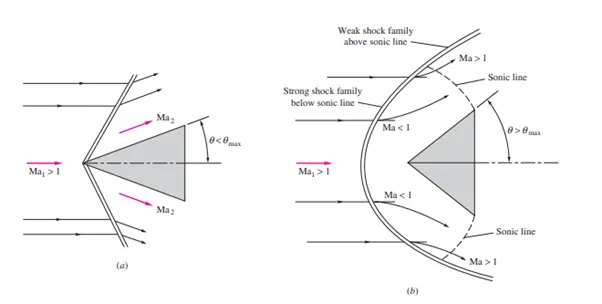
Supersonic flow past a wedge: (a) small wedge angle, attached oblique shock forms; (b) large wedge angle, attached shock not possible, broad curved detached shock forms

Prandtl Mayer Expansion waves

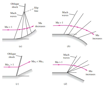
Below Figure shows four examples, one of which (c) fails the test for gradual changes. The gradual compression of (a) is essentially isentropic, with a smooth increase in pressure along the surface, but the Mach angle increases along the surface and the waves tend to coalesce farther out into an oblique shock wave. The gradual expansion of (b) causes a smooth isentropic increase of Mach number and velocity along the surface, with diverging Mach waves formed. The sudden compression of (c)cannot be accomplished by Mach waves: An oblique shock forms, and the flow is nonisentropic. This could be what we would see if we looked at (a) from far away. Finally, the sudden expanasion of d is isentropic and forms a fan of centered Mach waves emanating from the corner.

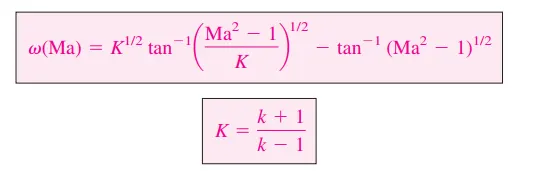
This is the Prandtl-Meyer supersonic expansion function and the change in angle is given by :

The angle
changes rapidly at first and then levels off at high Mach number to a limiting value as Ma →infinity.

The physical meaning is the angle through which the supersonic flow has to be expanded in order to obtain a given Mach Number at the downstream end.

Effect of SGS Parameter on SHOCK Location

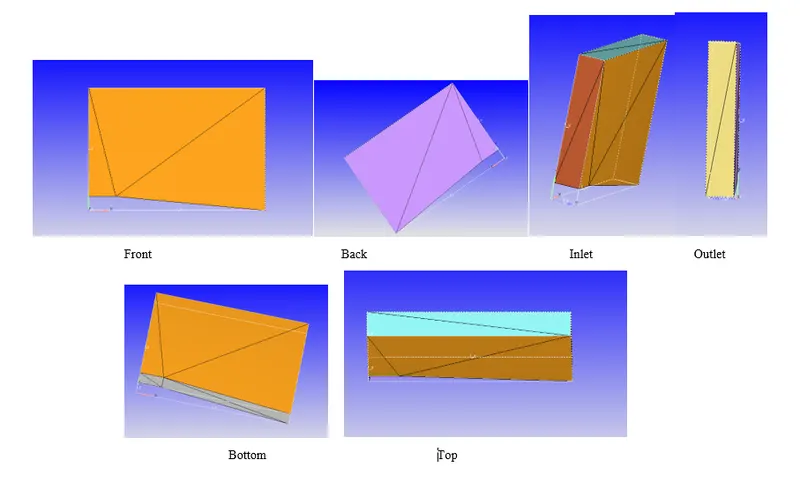
Boundary Zones:

Case Setup:

• In order to begin the case-setup, click on the case-setup and click begin case-setup and click Time based, since it is not a crank angle based like IC engines or Pumps but a steady-state channel flow setup.
• Then click on Materials and select Air to be predefined mixtures.
• Then open the Gas simulation and Global transport parameters and retain the default setting. And also retain the same setting for the species and Reaction mechanism.
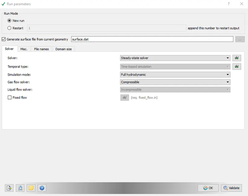
• Then click on the Run Parameter under the Simulation Parameter and choose the transient solver under the solver tab and then choose the Full Hydrodynmic under the simulation mode. And then choose the Compressible under the Gas flow solver.
• In the Miscellaneous tab, check the steady state monitor and uncheck the use shared memory because of we are running a steady state simulation flow here.
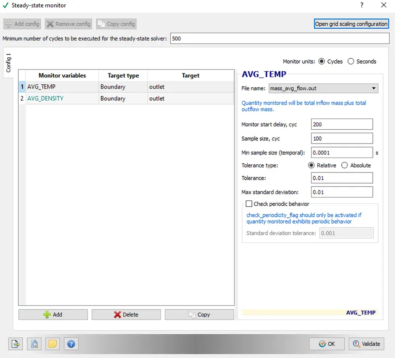
• Then click on the Steady-state monitor, click add config. And click Add to add the variables that needs to be monitored.

• The monitor start display is a parameter that ensures that the simulaion runs for a certain number of cycles before the variable can be monitored. This is especially useful in transient simulations when you want the solution to run for a particular amount of time before checking for convergence, if the steady state results are also required.
• Sample size denotes the number of cycles or seconds over which the variable is checked to see if the solution has converged. The solution is said to be converge when the average change over multiples iterations is less than the tolerance value. The tolerance value can be changed based on the problem and level of accuracy required.
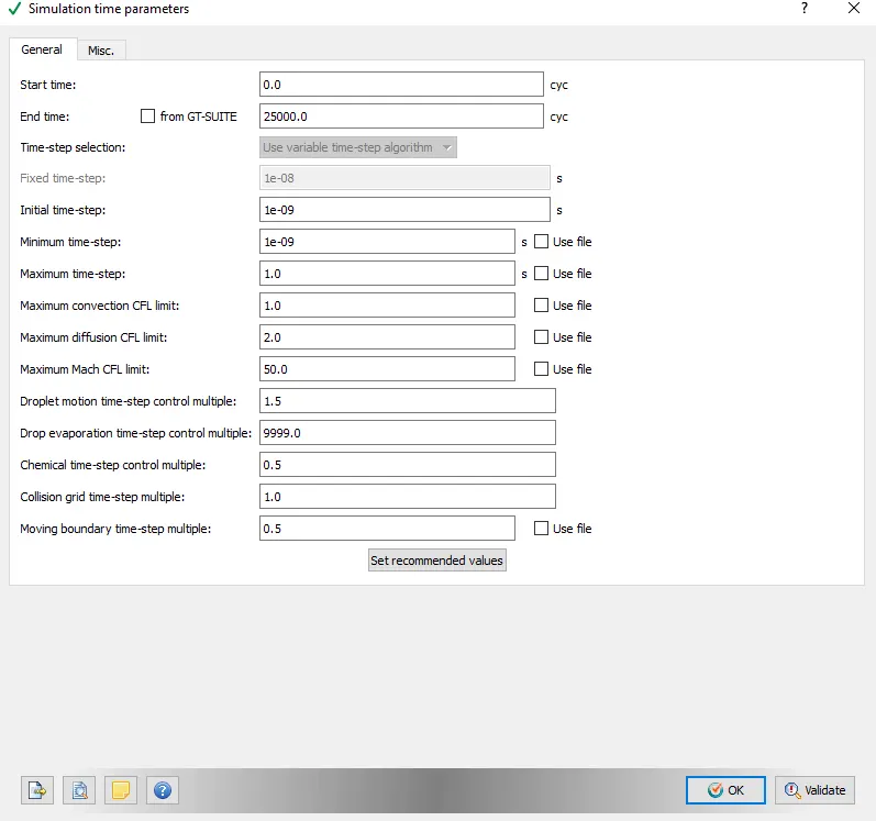
• In the simulation time parameter do the following changes.

Boundary Conditions:

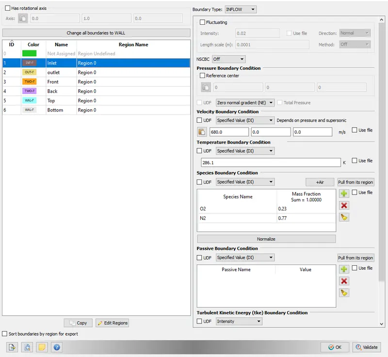
• At the inlet boundary we specify the velocity 680 m/s and select the predefined mixture as a Air which contains N2 as a 77% and O2 as 23%. And select the temperature to be specified of 286.1K. And we are taking the zero normal gradient(NE) for the pressure boundary condition at the inlet.

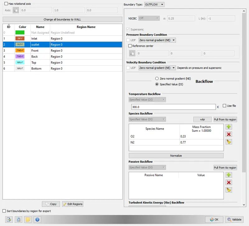
• At the outlet boundary, we specify the zero normal gradient boundary condition for both pressure and velocity. And give the temperature 300K at the outlet boundary.

• At the front and back wall, we are specify the 2d boundary condition.
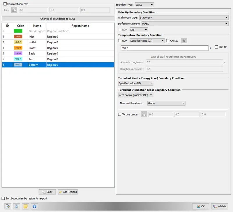
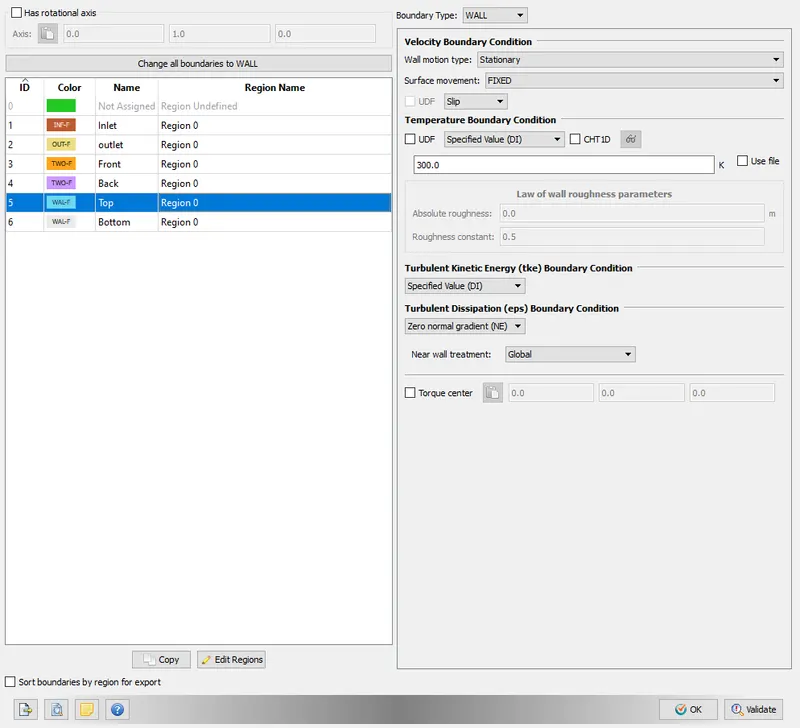
• At the top and bottom wall, we are taking the slip boundary condition.

Regions and Initializations:

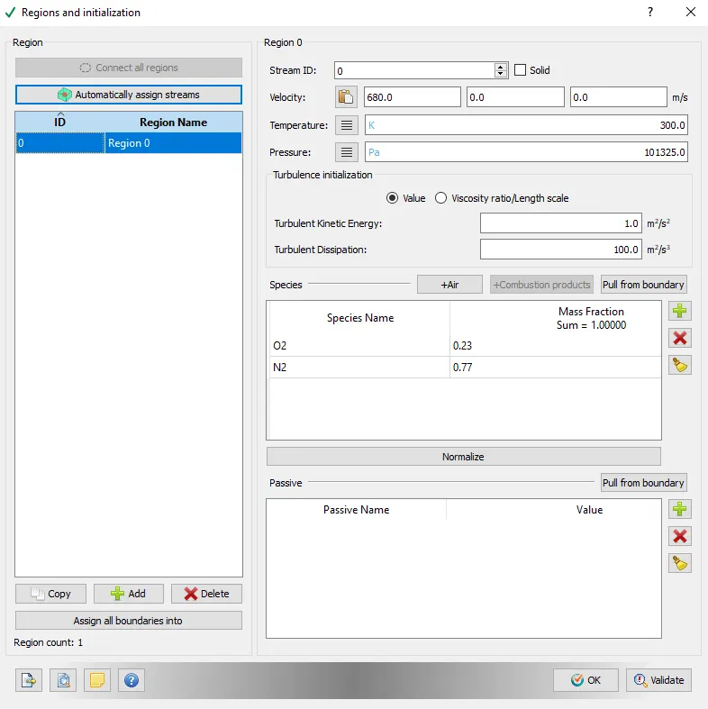
• In the grid control, the mesh size is in meters.

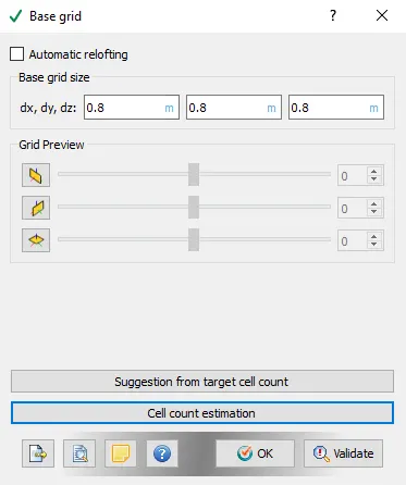
Meshing

Base grid of size 0.8 m is set in all directions. For capturing the details around the expansion waves, the base grid is further meshed around the shock with SGS 0.05 and 0.01. This is done through adaptive mesh refinement for adapting the accuracy of the solution within the sensitive or chaotic zones. When solutions are calculated numerically, they are restricted to some scale of quantified grids which is predetermined as in the Cartesian plane of the mesh.

Here in this project, sub grid scale of AMR is used on the Temperature, pressure and velocity fields. Two different sub grid scale of AMR SGS 0.05 and 0.01 is used inn the present study. The property helps to save computational cost by not meshing the base grid further and instead apply adaptive refinements. So, CONVERGE calculates these second order temperature, pressure and velocity fields and check the difference between the orders and gives the scope to refine the cells by proper embedding.

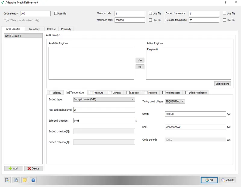
Size of the cell in scaled grid = (Size of cell in base grid) / 2^(amr_embed_temp_scale)

Base grid = 0.8m

amr_embed_scale = 2

size of cell in base grid = 0.8/2^2 =0.8/4=0.2m

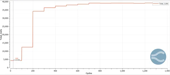
Case1: (converged in 7343 cycles; Computational Time: 83.89 s)

• With AMR SGS 0.05
• AMR Base: Temperature
• Embedding Level: 2

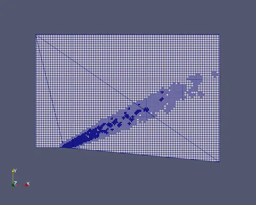
Mesh Cell Count

Case2 : (converged in 7302 cycles; Computational Time: 120.57 s)

• With AMR SGS 0.01
• AMR Base: Temperature
• Embedding Level 2

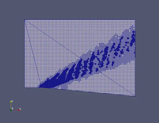
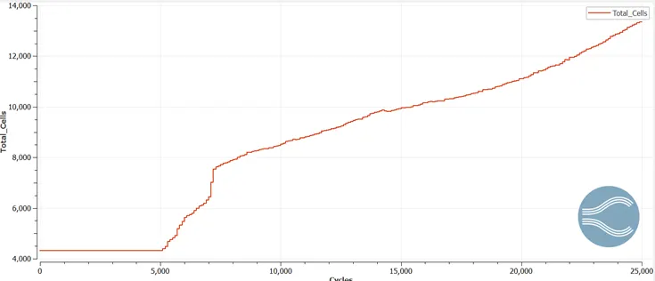
Mesh Cell Count

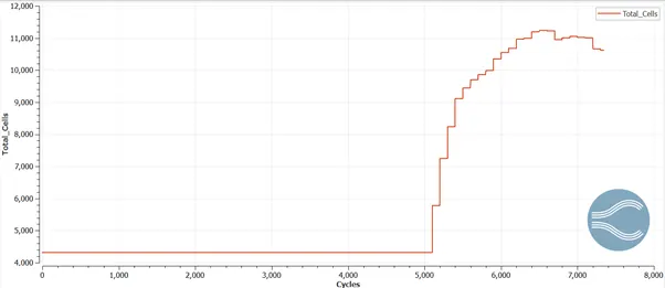
Case3 : ( Computational Time: 425.74667 s)

• With AMR SGS 0.01
• AMR Base: Temperature
• Embedding Level 2

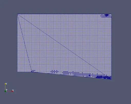
Mesh Cell count

Post Processing and Results

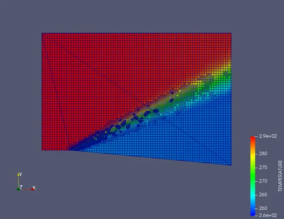
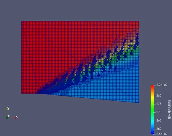
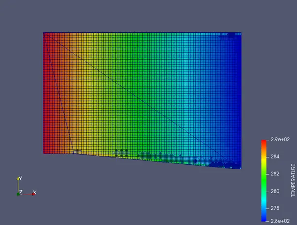
Velocity, density, Temperature and Pressure profiles have have been presented for both the cases for the given setup and is especially focused on the change of SGS parameter on the Expansion wave.

• Temperature contour plot:

Case1

Case 2

Case 3

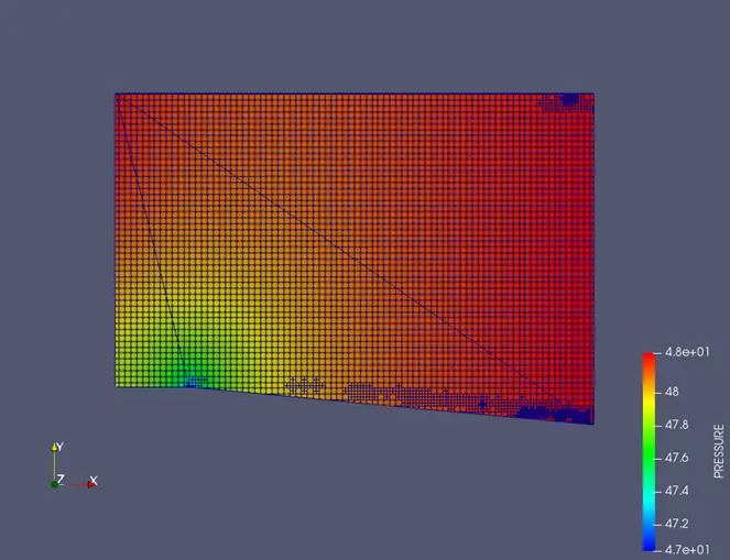
• Pressure contour

Case1

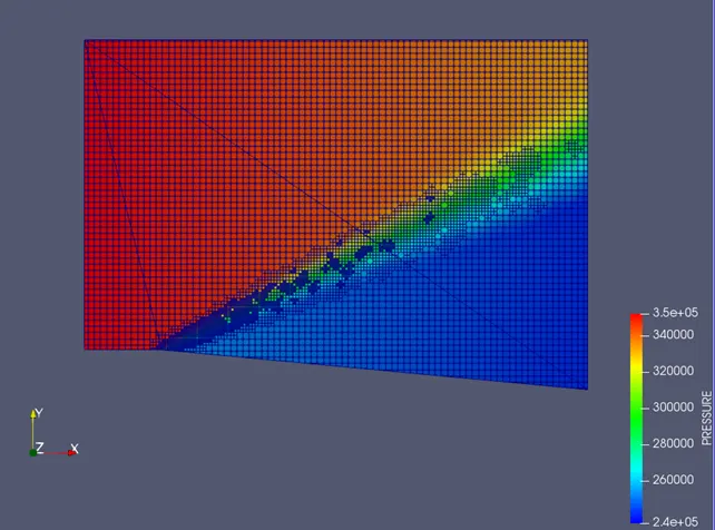
Case2

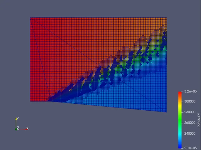
Case 3

• Velocity contour

Case1

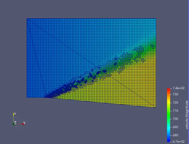
Case2

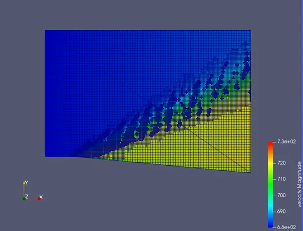
Case 3

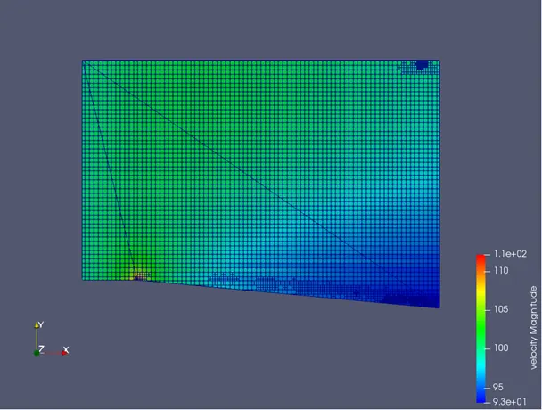
CASE1: SGS 0.05( Supersonic)

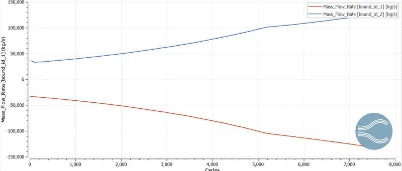
• Plots for Mass Flow Rate at inlet and Outlet

• Plot for static Pressure between the inlet and outlet

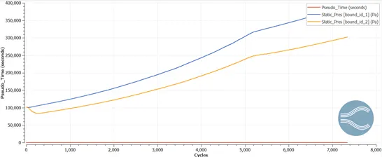
There is aconstant difference in the static pressure between the inlet and outlet. This is used for maintaining the flow at specified velocity.

The pressure decreases after the Shock i.e. (Upstream) D1 > D2 (Downstream)

The Expansion Shock relaxes the pressure.

• Plot for Average Mach Number between the inlet and outlet

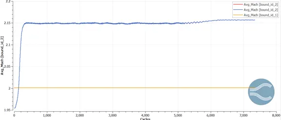
The average Mach Number at the inlet where the inlet velocity is 680 m/s and at the outlet the Mach No should be somewhat higher than that in the inlet and it is seen to be 2.15 whereas at the inlet it is 2. This allows us to have an idea of the angles between which the two shock waves exist.

The density decreases after the Shock i.e. (Upstream) D1 > D2 (Downstream)

The Expansion Shock relaxes the density.

• Plot for Average velocity at the inlet(680 m/s) and the outlet

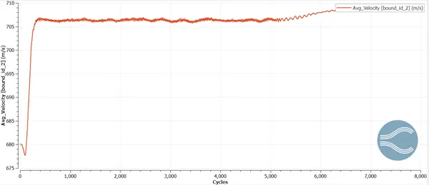
The average velocity jumps from 680 m/s to 706 m/s and fluctuates within 708 m/s and then attains a steady state which is in accordance with the phenomenon of supersonic flow.

• Plot for Average Temperature at the inlet and outlet

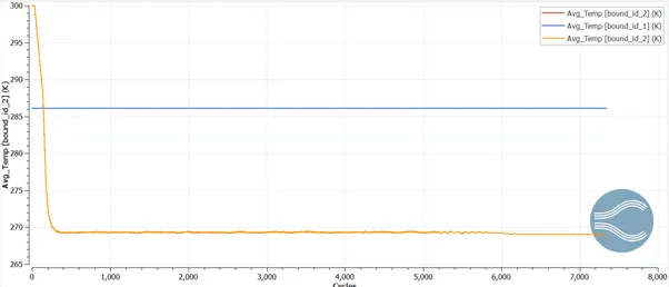
The average temperature shows the same trait as static pressure( with a constant difference between the inlet and the outlet). It decreases across the expansion fan and so is the case with average density.

The temperature decreases after the Shock i.e. (Upstream) T1 > T2 (Downstream)

The Expansion Shock relaxes the temperature.

• Plot for Average density at the inlet and outlet

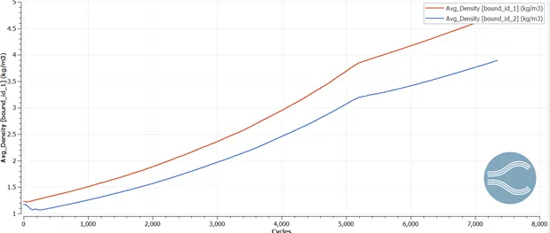
The density decreases after the Shock i.e. (Upstream) D1 > D2 (Downstream)

The Expansion Shock relaxes the density.

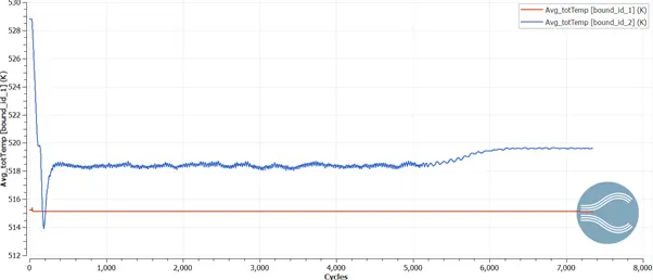
• Plot for total averaged Temperature at the inlet and outlet.

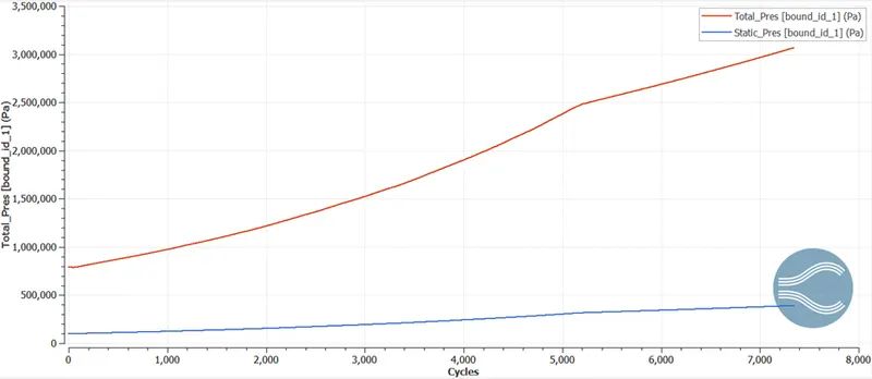
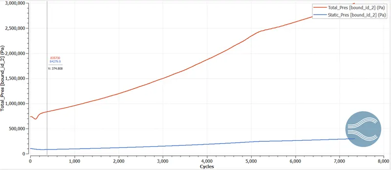
• Plot for Total pressure and Static pressure at the inlet and outlet

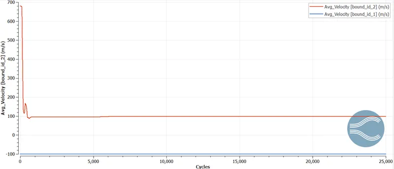
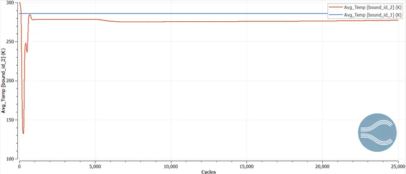
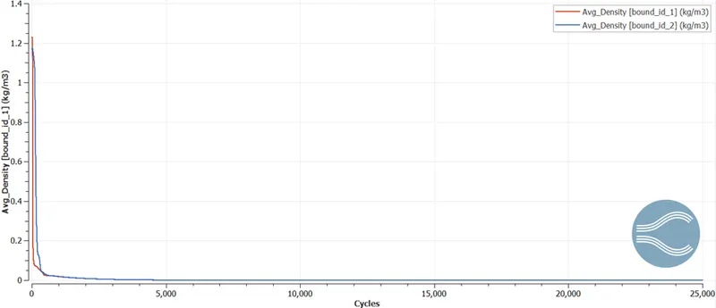
CASE 3: SGS~0.01(Subsonic) Inlet velocity-100 m/s

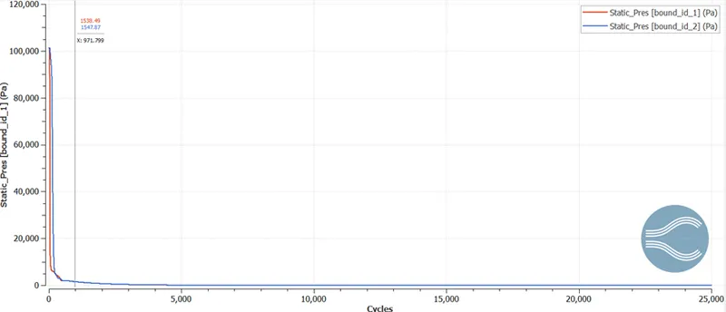
• Plot for static Pressure between the inlet and outlet

• Plot for Average Mach Number between the inlet and outlet

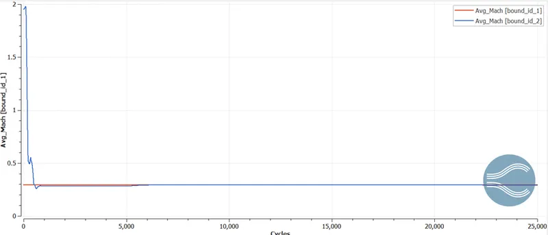
• Plot for Average velocity at the inlet(680 m/s) and the outlet

• Plot for Average Temperature at the inlet and outlet

• Plot for Average density at the inlet and outlet

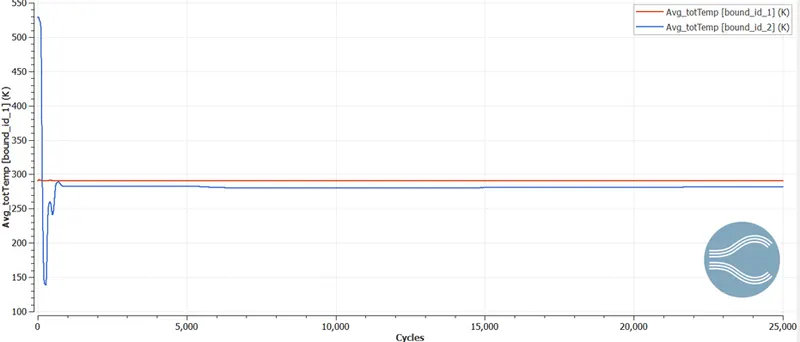
• Plot for total averaged Temperature at the inlet and outlet.

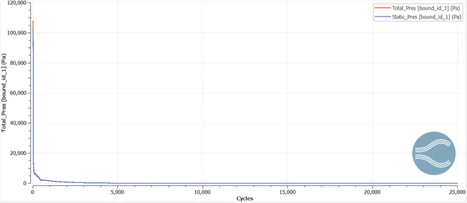
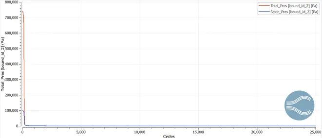
• Plot for Total pressure and Static pressure at the inlet and outlet

Animation

Temperature contour

• Case 1

• Case 2

• Case 3

Pressure contour

• Case 1

• Case 2

• Case 3

Velocity contour

• Case 1

• Case 2

• Case 3

CONCLUSION:

The supersonic and subsonic prandtl mayer expansion having a sharp corner was run in converge CFD in 3 cases(Cases 1 and 2 are for supersonic flow and Case 3 is for subsonic flow with an inlet velocity of 100 m/s). Various contours plots of velocity, pressure, density and temperature were studied and there were not so much difference ion the results other than the contour plots. While on the other hand there is a large difference observed in the mesh and the AMR with SGS 0.01 doesn't really work for the subsonic flow as there are no difference between the inlets and the outlets as we can see from the above plots

Changing the SGS values changes the number of cells that are formed during meshing and it is when Sub-grid temperature is greater than SGS value, the advanced refinement in the mesh occurs.

There is no major difference in the contour plots and the post processing results of SGS(0.01 and in 0.05) .

The inlet Mach no where flow enter to the geometry is 2 and the outlet mach no is 2.15 which correspond to an outlet velocity 708 m/s as compared to the inlet velocity 680m/s for the supersonic cases.

Effect of SGS parameter on shock location and total cell count

Cell Count: As the SGS parameter decreases, the total cell count increases i.e for small SGS parameter AMR refines the mesh for larger number of cells in the vicinity of the shock wave.

Shock Location: For high SGS parameter, the mesh refinement area or the area for theexpansion of fan is very small like (SGS = 0.01) and for the small SGS parameter, the mesh refinement area is larger.

In supersonic flow, the prandtl mayer expansion fan is clearly visible and the mesh refinement is also in the shock region. Whereas on the other hand , in the case of subsonic flow, the prandtl mayer shock fan is not clearly visible and even the mesh refnement is not visible. This is because there are no sudden fluctuations in pressure, velocity, temperature or density or in other words shock.Also the average Mach number inceases from the inlet to the outlet in case of supersonic flow and deceases in case of subsonic flow.