Week 5: Prandtl Meyer Shock problem

Aim: To simulate the Prantl Meyer Shock problem on Converge CFD.

• Types of Boundary conditions
• To understand the flow variation in a duct having a sharp corner.
• What is Shock?
• To study the effect of shock location variation based on SGS factor.

Dirichlet boundary conditions

In computational fluid mechanics, the classical Dirichlet boundary condition consists of the value of velocity and/or pressure to be taken by a certain set of nodes. It is common to refer to some sets of b.c. according to the following terminology:

• slip boundary condition: the velocity normal to the boundary is set to zero, while the velocity parallel to the boundary is let free
• no-slip boundary condition: both the velocity normal to the boundary and the velocity parallel to the boundary are set equal to zero.

At least one homogeneous b.c. on the pressure (i.e. p=0) has to be imposed as a reference for open domains, for instance, in the highest boundary of the air domain.

Neumann boundary conditions

Constraints on the derivative of velocity or pressure fields are mainly used in two cases. The first case is the application of a symmetry plane, thus:

`(delu)/(deln) =0`

Since this condition is always applied in addition to a Dirichlet b.c. it is naturally satisfied. The second application is the modeling of wall friction, in the case when it is proportional to the strain rate:

`S= (nablau+ nabla^T u)`

Robin boundary conditions

It is used to describe semi-reflective walls, which partially absorb waves. It is not a very common application and it can be used only for pressure-based models. It is mostly used for acoustic applications.

THE PRANDTL MEYER EXPANSION FAN:

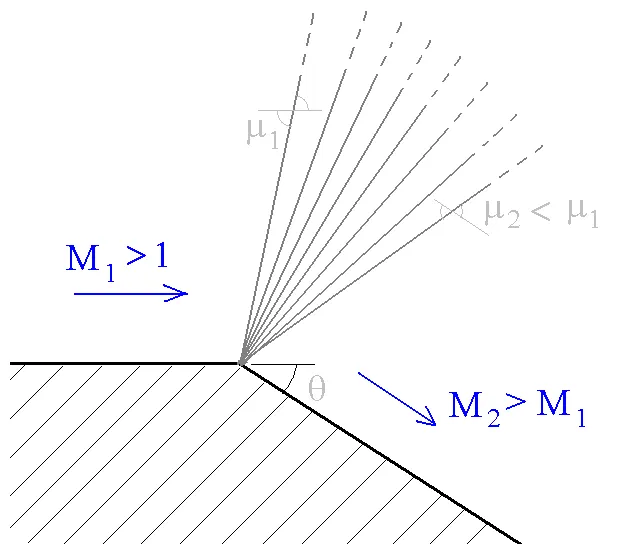
A supersonic expansion fan, known as Prandtl–Meyer expansion fan, a two-dimensional simple wave, is a centered expansion process that occurs when a supersonic flow turns around a convex corner. The fan consists of an infinite number of Mach waves, diverging from a sharp corner. When a flow turns around a smooth and circular corner, these waves can be extended backwards to meet at a point. Each wave in the expansion fan turns the flow gradually (in small steps). It is physically impossible for the flow to turn through a single "shock" wave because this would violate the second law of thermodynamics.

What is a Shock Wave?

A shock wave, or shock, is a type of propagating disturbance that moves faster than the local speed of sound in the medium. Like an ordinary wave, a shock wave carries energy and can propagate through a medium but is characterized by an abrupt, nearly discontinuous, change in pressure, temperature, and density of the medium.

Case Setup:

Procedure to setup the case:

• Select time based in the application.
• We select Air as the premixture in the material section of the setup tree. We must also ensure that the simulation type is gas.
• In the simulation parameters, we select the stead solver and make sure that the type of simulation is full hydrodynamic. (Usually, simulations are run in non-hydrodynamic mode to ensure that the grid formed on the case is as expected. Due to the simplicity in the geometry, we directly use the full hydrodynamic mode.)
• We setup the boundaries as required also we assign the region to each of the boundary.
• Here we employ the turbulence modeling where we use the RANS method and we use the RNG k ε.
• The most important aspect in this model is to make sure that the model is dimentioned in meters. Also the base grid dimensions are to be mentioned in meters.
• In order to study the phenomenon of shock, we employ the adaptive mesh refinement and set the SGS to required values to study this phenomenon.
• The post processing is done on the results once the simulation is complete.

Few particulars

Velocity at inlet: 680m/s

velocity at outlet: Zero Normal Gradient (NE)

Temperature Boundary condition: 300K

Top and Bottom walls: Slip

Species Boundary conditions:

O2= 23%

`N_2`=77%

Simulation parameters

Total number cycles= 25000 cyc

minimum time steps=1e-7s

maximum time step=1s

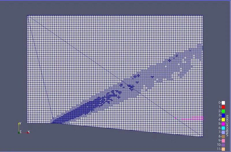
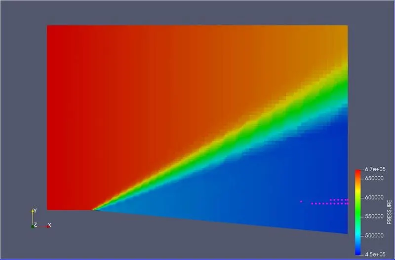
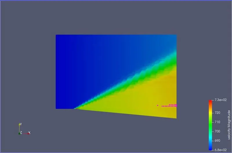
Case 1: Inlet velocity: 680 m/s and SGS 0.05

Pressure profile:

Velocity profile:

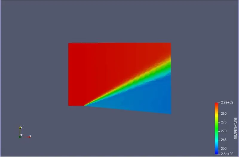
Temperature Profile:

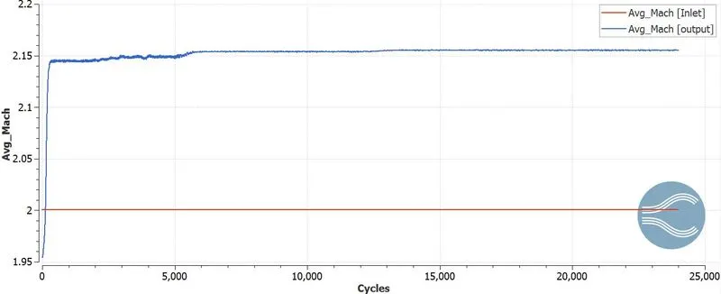
Plot for mach number:

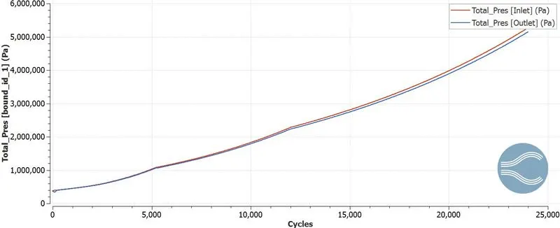
Plot for total pressure:

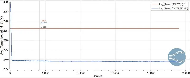
Plot for average temperature:

Number of Cells:

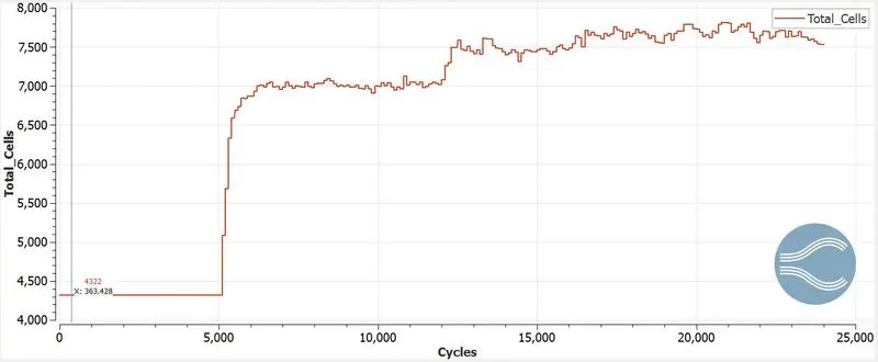
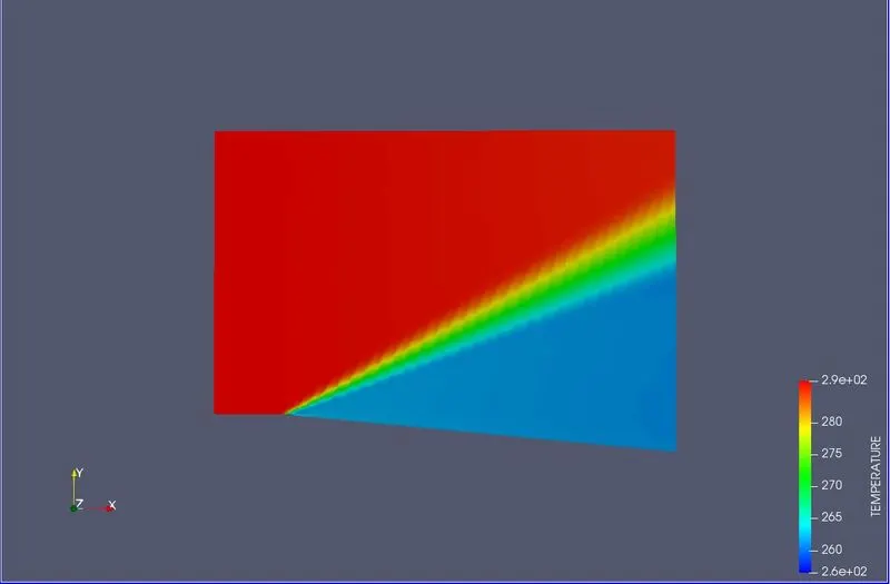
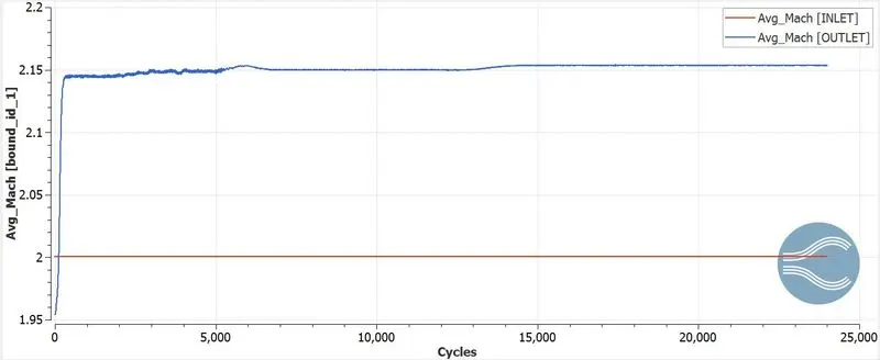
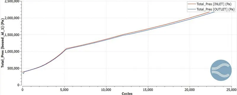
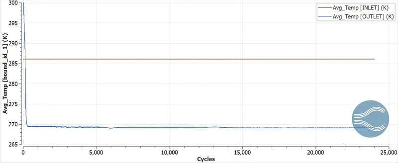
Case 2: Inlet velocity: 680 m/s and SGS 0.01

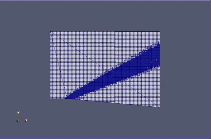
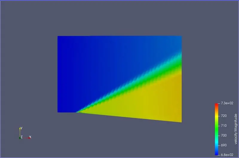
velocity profile:

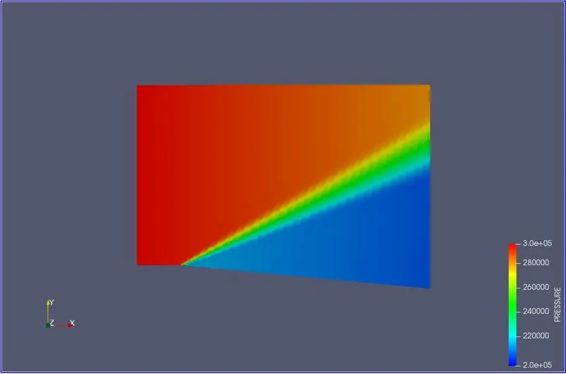
Pressure profile:

Temperature Profile:

Plot for mach number:

Plot for total pressure:

Plot for average temperature:

Number of Cells:

Inference:

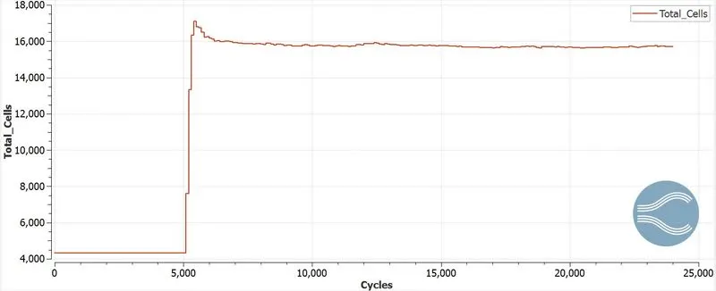
1. From the plots, we can observe that the simulation attains steady state at about 6000 - 7000 cycles for the 1st case whereas in the second case it attains it in about 5000 cycles.
2. From the profiles we can observe that the shock was better captured in the case with lower SGS (ie. sgs=0.01). This is because the refinement level is much higher in the case of a lower SGS value.
3. A significant difference was observed in the total number of cells. The number of cells in case 2 was observed to be higher as the refinement was significantly higher than the former. This enables for better results.
4. As per the location of shock wave was observed, case 2 had a larger bandwidth of the shockwave. The wave was pronounced than the former thus capturing the shock appropriatly.
5. From the above we can infer that the lower the SGS the better the solution.

REFERENCES:

https://www.simscale.com/docs/simwiki/numerics-background/what-are-boundary-conditions/

https://en.wikipedia.org/wiki/Prandtl%E2%80%93Meyer_expansion_fan