Prandtl Meyer Shock simulation using Converge CFD

Objective:

• Simulate the Prandtl Meyer shock wave using Converge and post-process the results using Paraview.
• Study the boundary conditions used in shock problems
• Study the effect of SGS parameter on shock location

Types of boundary conditions

Dirichlet BC

It is a type of boundary condition in mathematics. It specifies the values that a solution needs to take along the boundary of the domain.

Eg: Velocity inlet

Neumann BC

Neumann BC is a type of boundary condition. When imposed on an ordinary or a partial differential equation, the condition specifies the values in which the derivative of a solution is applied within the boundary of the domain.

Mixed BC

It is the combination of Dirichlet and Neuman boundary conditions

Shock wave

A shock wave is a type of propagating disturbance that moves faster than the local speed of sound in the medium. Like an ordinary wave, a shock wave carries energy and can propagate through a medium but is characterized by an abrupt, nearly discontinuous, change in pressure, temperature, and density of the medium.

When the speed of a source exceeds the speed of sound (v > c) the wave fronts lag behind the source in a cone-shaped region with the source at the vertex. The edge of the cone forms a supersonic wave front with an unusually large amplitude called a "shock wave".

Case setup

Geometry

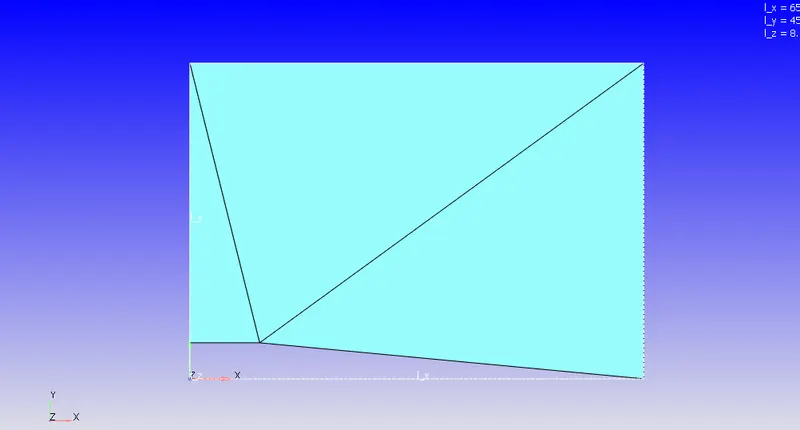
Material

Predefined mixture: Air

Species: N2, O2

Solver: Steady-state solver

Navier stokes solver type: Density-based

Turbulence modeling: RNG K epsilon

Boundary conditions

Inlet: Inflow BC

Inlet velocity=680 m/s

Outlet: Outflow BC

Pressure BC= Zero normal gradient

Velocity BC=Zero Normal Gradient

Front and back: Two D BC

Top and Bottom: Wall BC

Wall motion type: Fixed

Regions and initialization

Air is added

O2=0.23

N2=0.77

Meshing

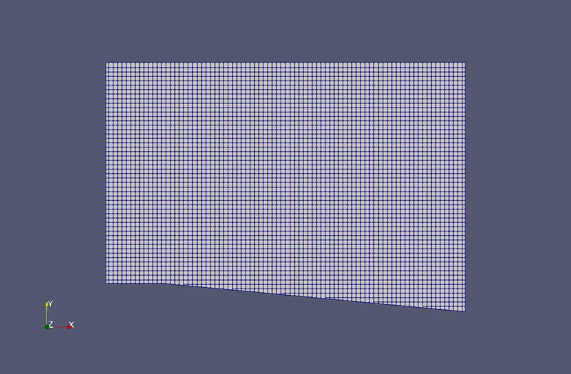
Base size=0.8 m

Temperature-based adaptive mesh refinement is added. In order to find out the effect of subgrid-scale temperature on shock location, The simulation is run for two different SGS value.

Case-1

Maximum embedding level=3

SGS temperature=0.05 K

Case-2

Maximum embedding level=3

SGS temperature=0.03 K

Simulation parameters

Start time=0 cyc

End time=25000 cyc

Initial timestep=1e-06s

Maximum timestep=1 s

Simulation Mode: Full hydrodynamic

Output files

The time interval for writing 3D output files=250 cyc

So the solver writes a 3D output files after every 250 cycles.

Post-processing

Velocity contour

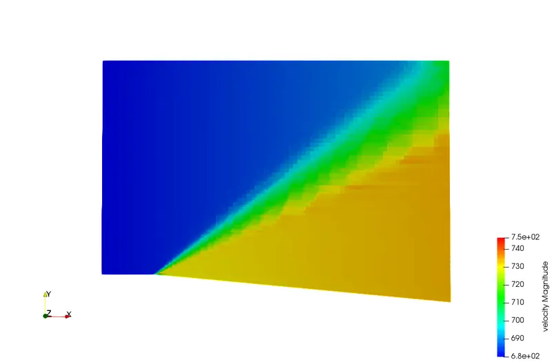
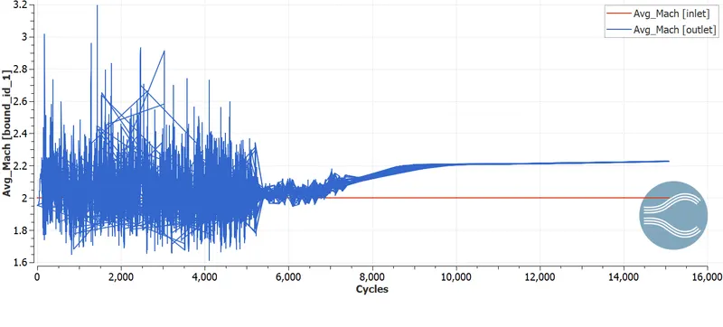
Across the expansion fan, the flow accelerates, and velocity increases and Mach number increases. From the velocity contour, we can see that velocity is high near the outlet. The increase in Mach number is shown in the plot below,

Pressure contour

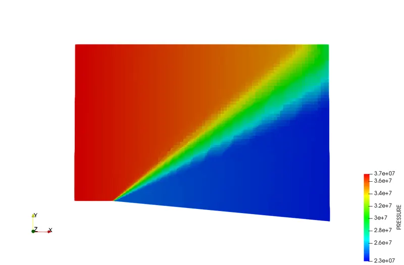
Static pressure decreases across the expansion fan. From the pressure contour we can see that near the outlet pressure is low and in the inlet region pressure is high.

Temperature contour

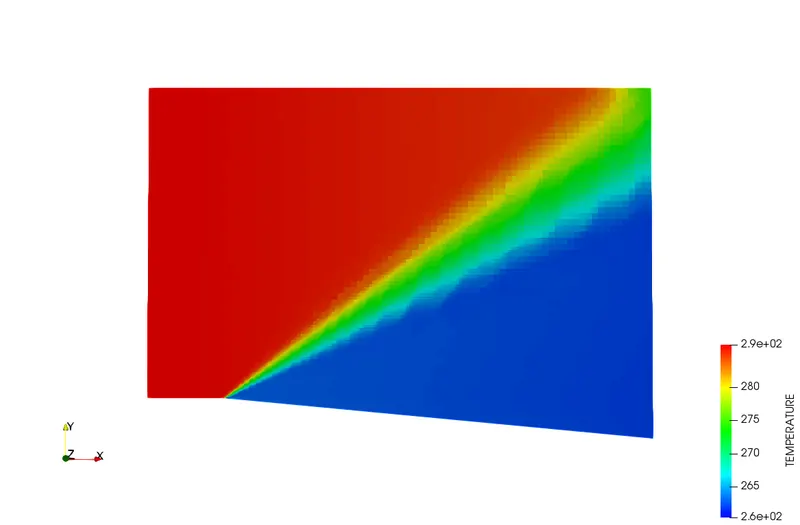
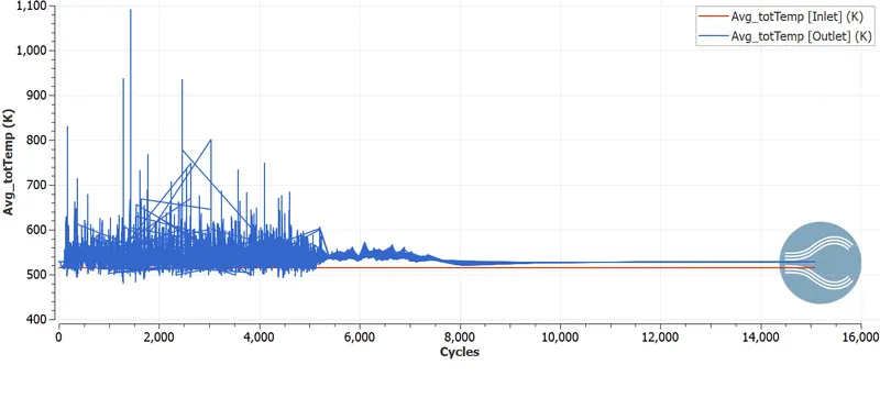
Temperature also decreases across the expansion fan. Since the process is isentropic, the stagnation properties (e.g. the total pressure and total temperature) remain constant across the fan. It is shown in the plots below,

Effect of SGS temperature

Temperature animation

Temperature animation with adaptive mesh refinement for two different values of subgrid-scale temperature is shown below,

Case-1[SGS=0.05K]

Case-1[SGS=0.03K]

Temperature plot with AMR[Case-1]

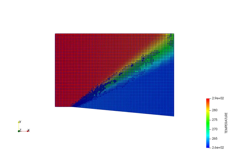
Temperature plot with AMR[Case-2]

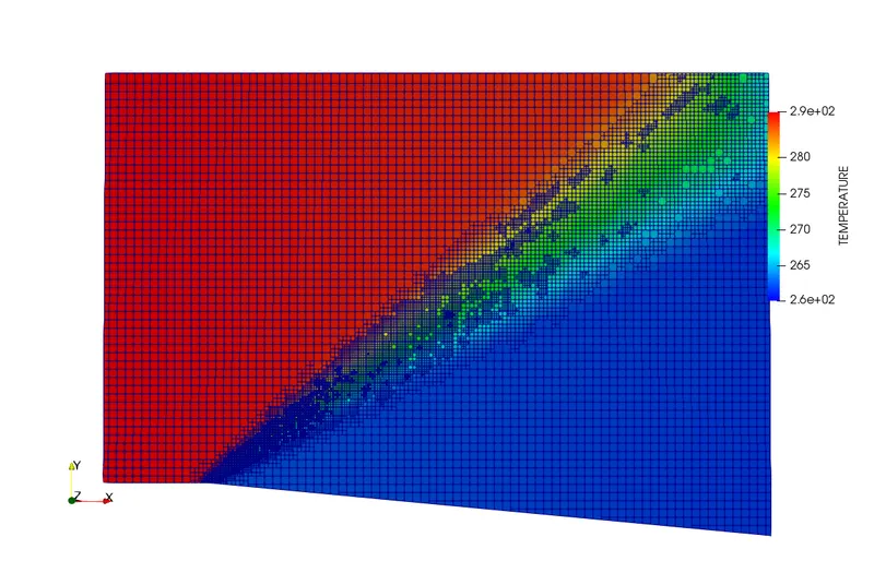
When the SGS value decreases more cells are created in the shock region where the temperature change occurs. The total cell count plot for the two cases are given below,

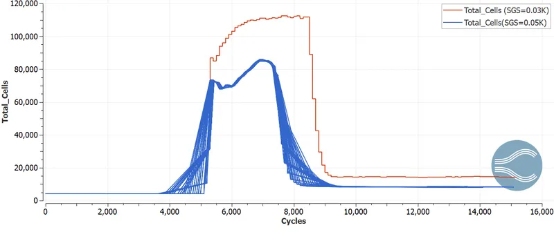
From this, we can see that number of cells increases with a decrease in SGS temperature value.

Conclusion

• The Mach number at the outlet is greater than the Mach number at the inlet.
• Across the expansion, fan flow accelerates and temperature, static pressure decreases.
• Since the flow is isentropic stagnation properties remain constant across the fan
• The mesh becomes more refined with a decrease in SGS temperature. And the number of cells increases. The total number of cells for different values of SGS temperature as per the above simulation

SGS=0.05 K, Total number of cells=8190

SGS=0.03 K, Total number of cells=14572