Week 5: Prandtl Meyer Shock problem
AIM:
Prandtl Meyer Shock problem
objectives:
1. Shock flow boundary conditions
Do a literature search on what BC's are typically used for shock flow problems
2. What is a shock wave?
In your own words, describe the physics behind shock waves
3. Effect of SGS parameter on shock location
In the Prandtl Meyer shock problem, look at the effect of SGS temperature value on cell count and the shock location
theory:
shock wave-
when an aeroplane flying welll below the speed of the sound creates a disturbance in the air and sends out pressure pulses in all directions as shown in below figure (a) . air ahead of aeroplane receives these messages before the aeroplane arrives and the flow seprates around the aeroplane, but as the aeroplane approaches the speed of the sound. the pressure pulses merge closer and closer together as shown in below figure (b) in front of aeroplane and little time elapses between the time the air gets the waning of the aeroplane approch and aeroplane's actual arrival time. at the speed of the sound the pressure pulses move at the same speed as the aeroplane as shown in below figure (c). they merge together a head of aeroplane into a shock wave which is an almost instantaneous line of change in pressure, temperature and density.
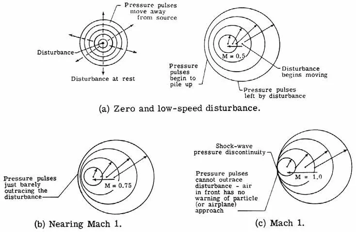
the air has no warning of the impending approach of the aeroplane and abrutply passes through the shock system. there is a tendency for the air to break away from the aeroplane and not flow smoothly about it. as a result there is a change in aero dynamic forces from those experienced at low incompressible low speeds.
prandtl meyer expansion fan-
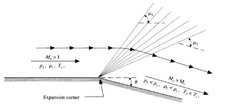
As an object moves through a gas, the gas molecules are deflected around the object. If the speed of the object is much less than the speed of the sound of the gas, the density of the gas remains constant and the flow of gas can be described by conserving momentum and energy. As the speed of the object increases towards the speed of sound, we must consider compressibility effects on the gas. The density of the gas varies locally as the gas is compressed by the object. When an object moves faster than the speed of the sound, and there is an abrupt decrease in the flow area, shock waves are generated. If the flow area increases, however, a different flow phenomenon is observed. If the increase is abrupt, we encounter a centered expansion fan. The word "expansion" denotes that the area is increasing. There are some marked differences between shock waves and expansion fans. Across a shock wave, the Mach number decreases, the static pressure increases, and there is a loss of total pressure because the process is irreversible. Through an expansion fan, the Mach number increases, the static pressure decreases and the total pressure remains constant.
BC's are typically used for shock flow problems-
here i have taken neumann boundary conditions at outlet of the geometry. in neumann boundary conditions, the normal derivative of a function is specified. i have taken this boundary condition because the values of the primitive variables are not there before solving of the prolem. initially the normal derivative of the variables are defined as zero normal gradient. in a supersonic flow, we cannot take the certain primitive variables at outlet because the compressibility effects also we need to consider. if we taken certain values means the solution gets diverged.
geometry:
after opeing the converge. drag the stl file fro the file manager
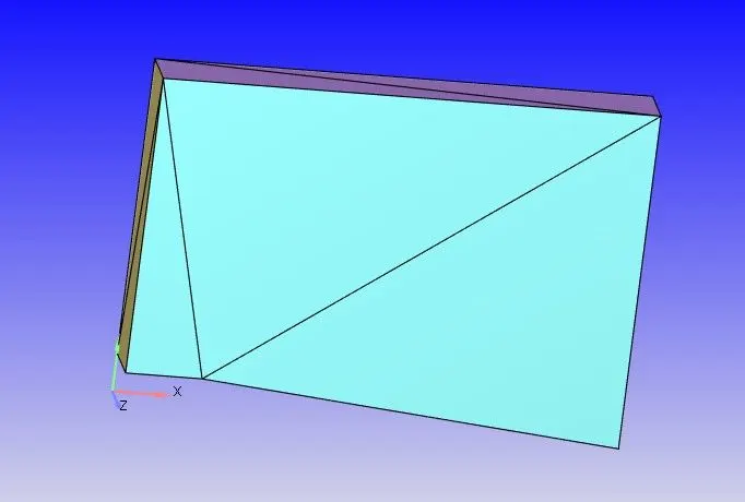
now use the boundary flagging option, name the boundaries of the surface of the geoemetry.
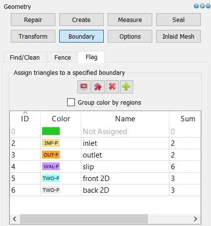
in the above figure, sum represents the number of triangles selected at the each boundary. now use normal toggle tool. in the converge,the normals are aloways directed to outside of the box faces as a default. but here the fluid is inward flow. so eliminate them, click on transform in geometry and slect of triangle and click apply. to check whethere the geometry is correct or not(ie open edges errors, overlap errors), click on the diagnosis which is shown at the bottem left of the display and click findings. mow buid the case setup.
case setup:
application type: time beased
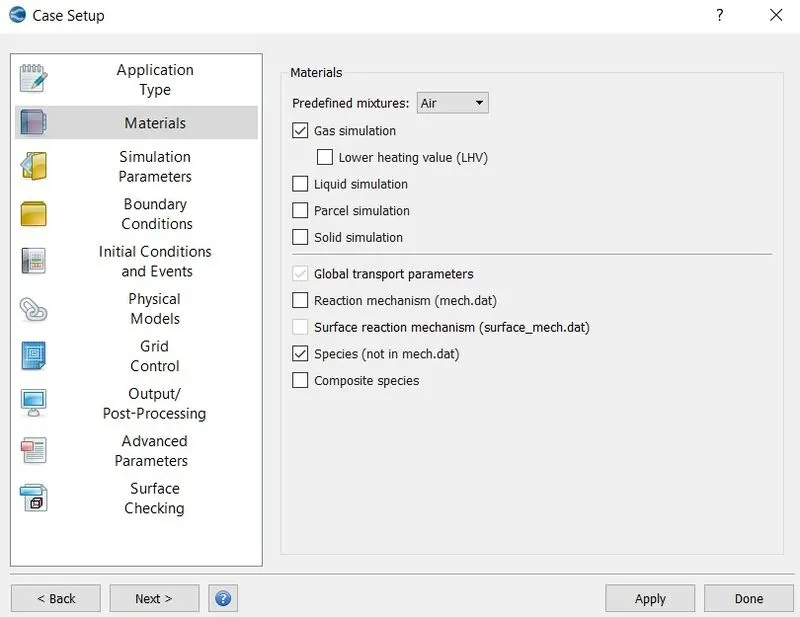
materials: air
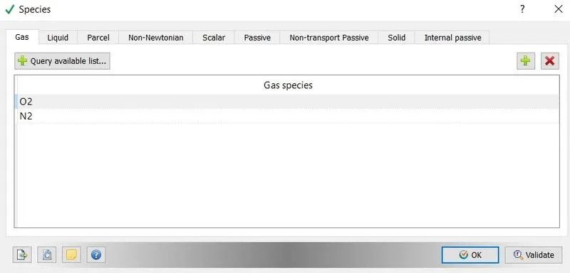
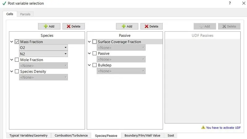
click on gas simulation as the air is gaseous state and click on species to calcuate how the mass fraction of N2 and O2 are changing along the flow.
species-
simulation parameters:
run parameters-
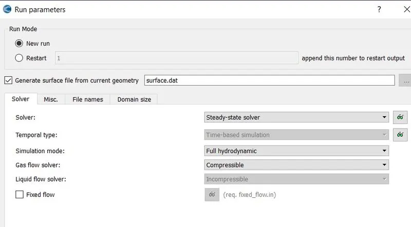
i am running the somulation using steady state solver. full hydrodynamic simulation mode is used for simple geometries.
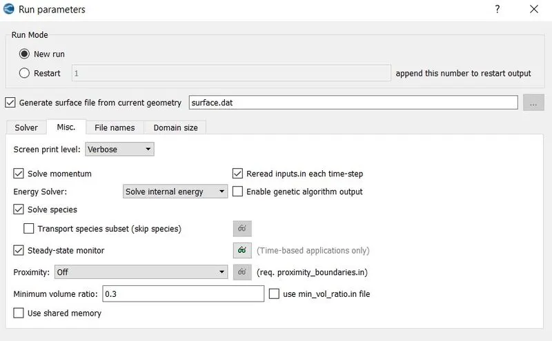
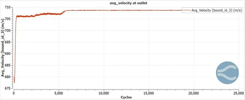
- steady state moniter- it moniters the primitive variables wheather they reached the steady state or not. minimum number of cycles to be executed for steady state solver is 10000. it tells that even if we give the number of cycles to run the simulation at 25000, the software stop calculating the simulation if it reached the steady state in between 10000 and 25000 cycles. moniter start delay indicates the software starts monitering that the solutions whether converged or not.. simple size indicates the soft ware takes the solution for every 1000 cycles and compar the difference in changing of primitive varisbles to see whether they reached steady state or not.tolerence denotes the diference in changing of primitive variables at every 1000cycles.
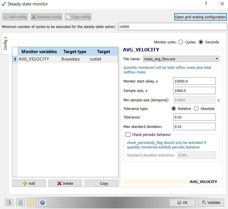
simulation time parameters-
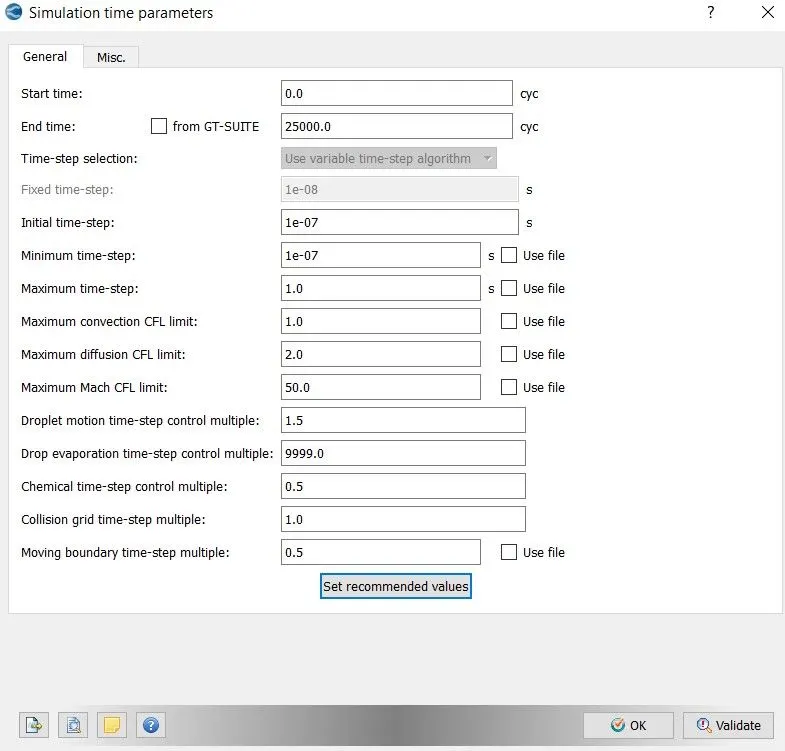
solver parameters-
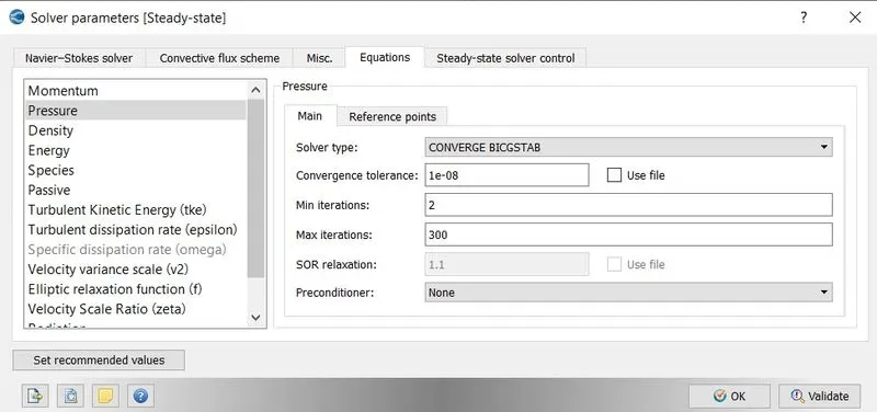
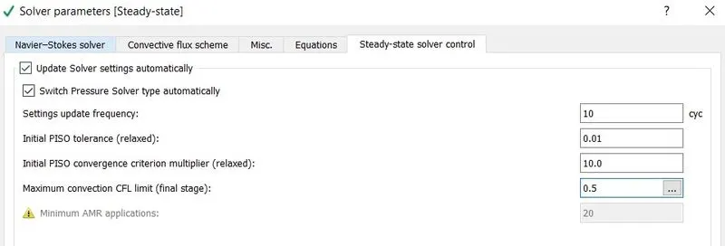
pressure based solver is used here and the max. cfl number taken is 0.5
initial conditions and events:
regions and initialization-
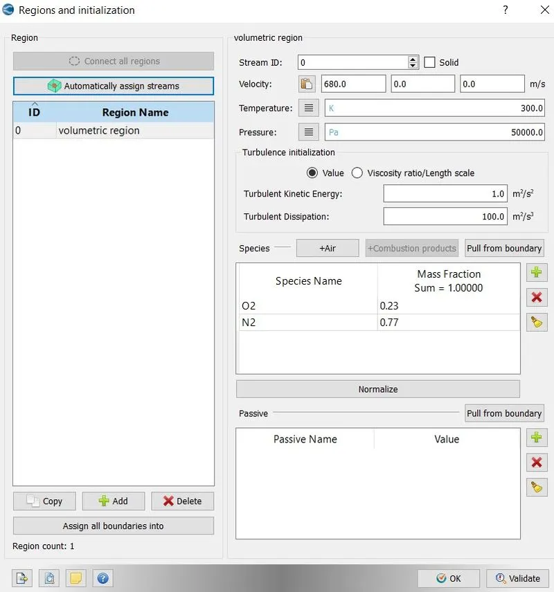
here i have named the entire box region as volumetric region. initially the temperature and pressure of the air at all the cells are taken as below.
boundary conditions:
boundary-
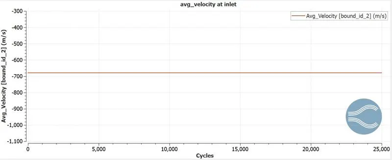
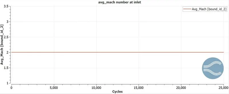
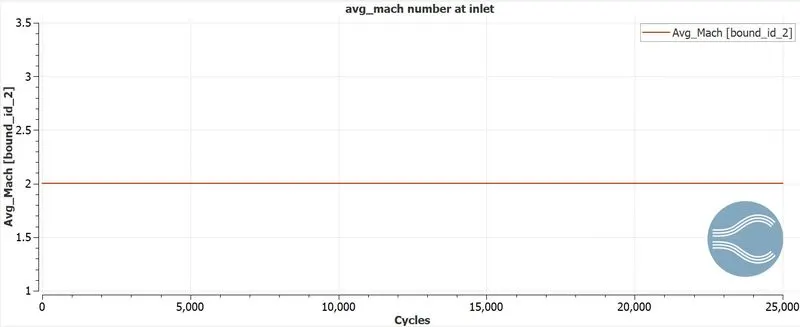
- inlet- the inlet velocity i have taken is 680 m/s. the pressure boundary condition i have taken is zero normal gradient. initial temperature of the air is 286.1 k . i have taken this because the speed of the sound at temperature 286.1 k is 340 m/s. so it means the mach number at the inlet i have taken is 2 which is supersonic flow.
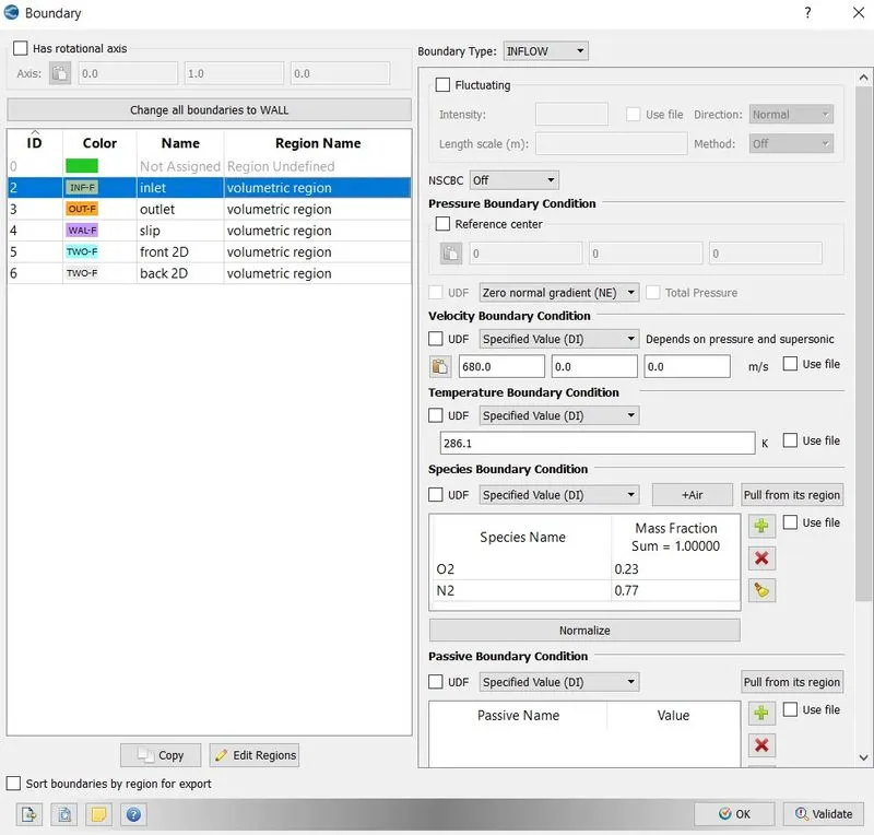
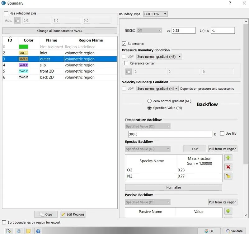
- outlet- at the outlet pressure boundary i have taken is zero normal gradient
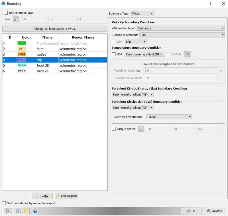
- slip - the top and bottem walls are named as slip.
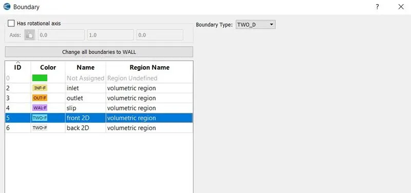
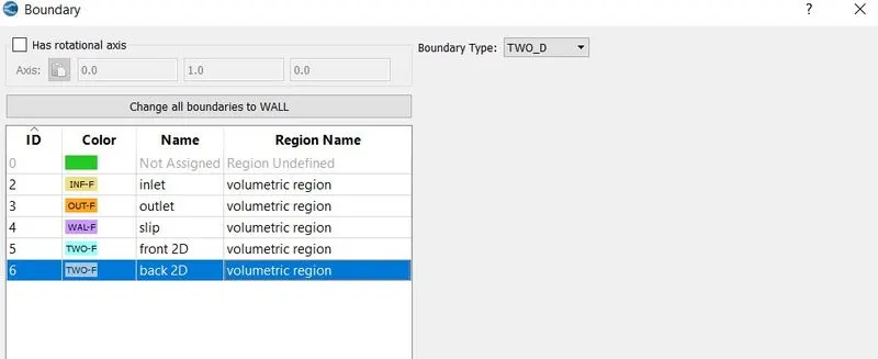
- front 2D and back 2D-
grid control:
base grid-
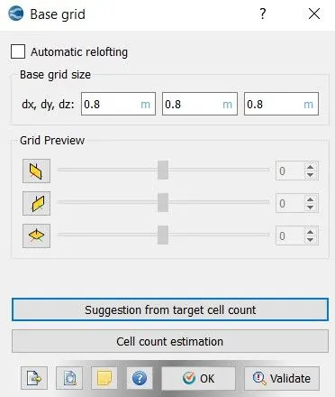
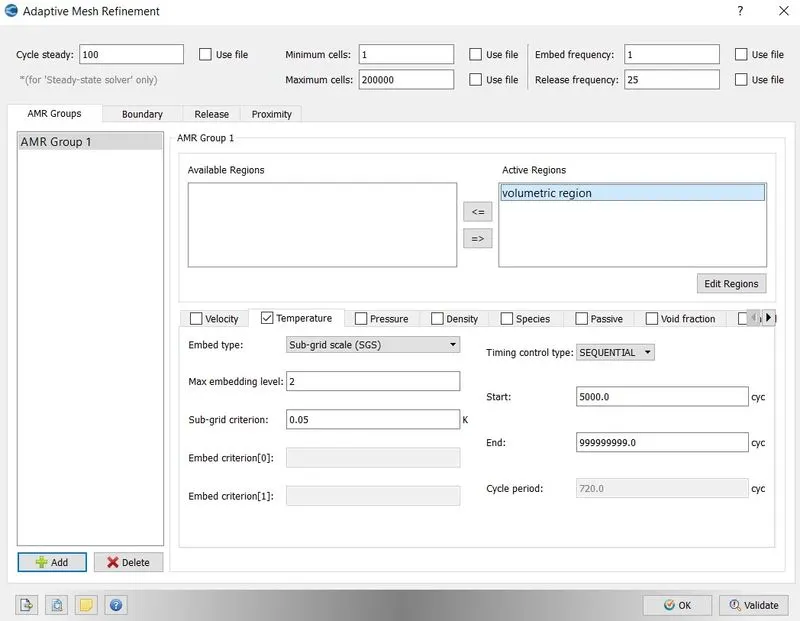
adaptive mesh refinement-
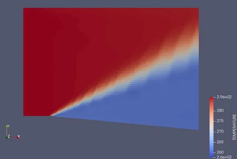
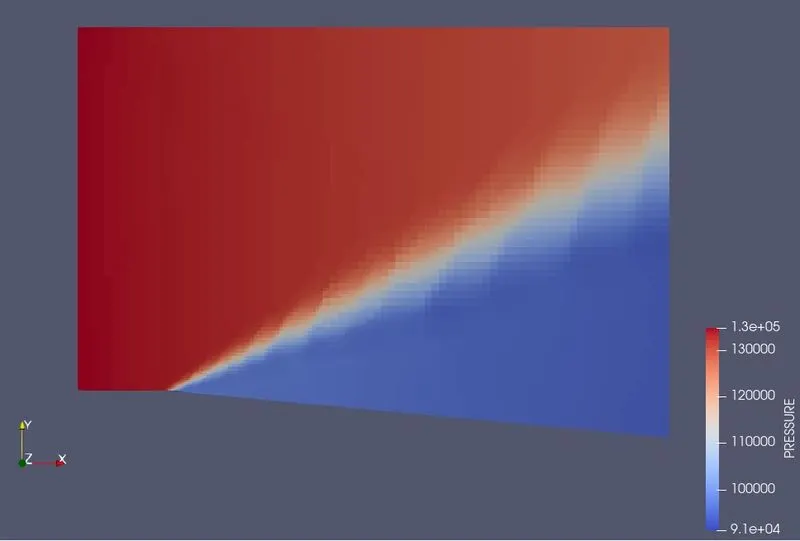
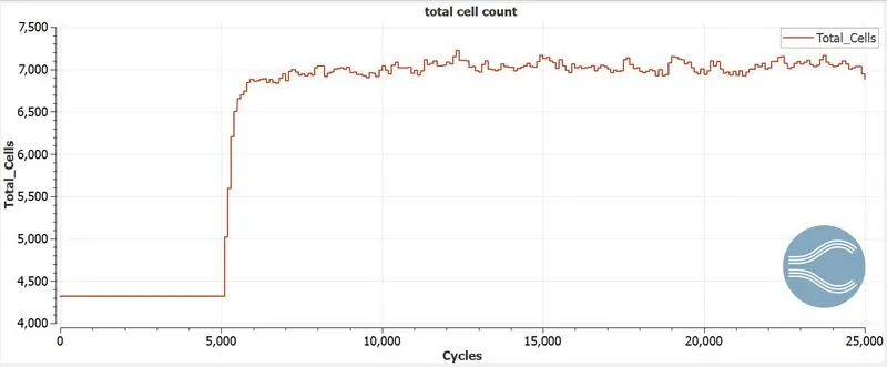
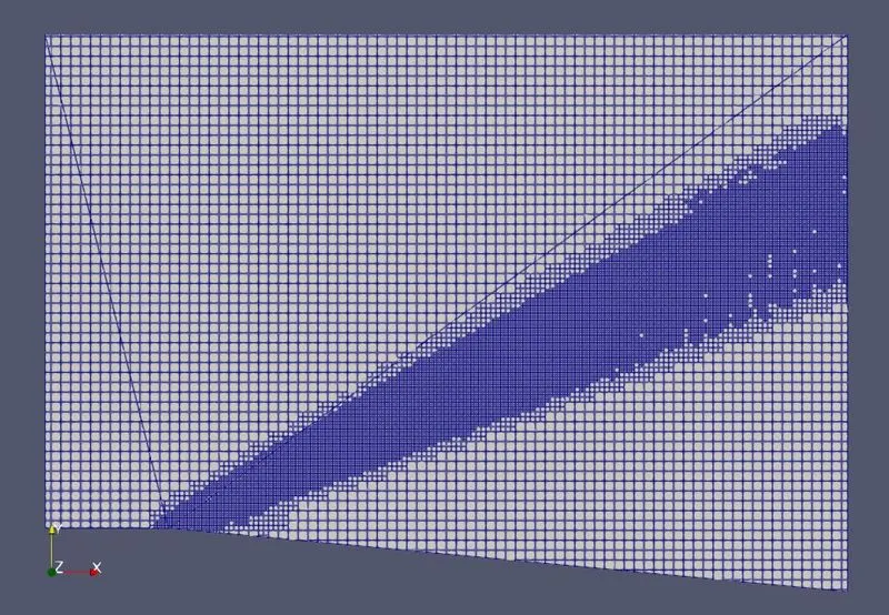
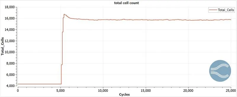
adaptive mesh refinement option is used to refine the mesh in the areas where the second order derivative of primitive variables is fluctuates more than the sub grid criteria. here i have taken the primitive variable is temperature. the sub grid criteria is also calles SGS parameter. the maximum embedding layers means the number of layers of cells that can be refined during the fluctuations of the temperature to visualize the pressure waves clearly. we kow that pressure wave is termed as shock wave. to visualize the shock wave i have refined the cell size using adaptive mesh refinement.
output/post-processing:
post variable selection-
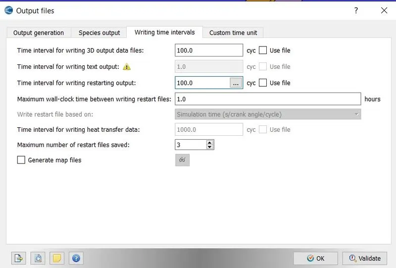
output-
solution:
now export all the input files in a folder. so from this we can see that converge is used to create the input files for the simulation. now insert the two application files from the converge folder to the folder where i have exported all the input files.

for the simulation i have used cygwin64 terminal. in cygwin termpinal open the folder where you have pasted all the input and application files.
now for the simulation write mpiexec.exe -n 4 converge.exe restricted and click enter. here 4 represents the number of processors used at a time.
post processing of results:

for this copy post convert application from converge folder to output folder which is generated in the input files folder. we are doing this because we are goingto convert all the output files into a vtk file which can be easily read by paraview software. toconvert the files we have to use post conver application as shown in the figure. there we can see the results that are obtained. now in cygwin open the output folder and write mpiexec.exe -n 4 post_convert.exe and click enter. now the below figure will appear
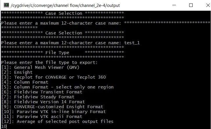
after naming the case and choosing 10, hit enter. now click yes for boundary output surface. now all the output files will appear and then write 'all' to convert all the output files. now select 'all' at cell variable selection menu. now all the files gets converted into varaview vtk files.
now open paraview. in paraview, open file and select case name .. vtm file which is present in the output files. finally we see the geometry in the paraview. now choose slice tool to select the axis along which all the primitive variables are same. as we know that, along z axis the primitive varibles are equal. so select axis and click apply.
case a:
velocity 680 m/s and with SGS parameter 0.05 k
grid-
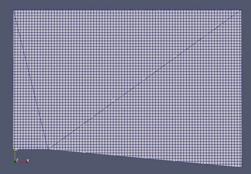
final grid after simulation-
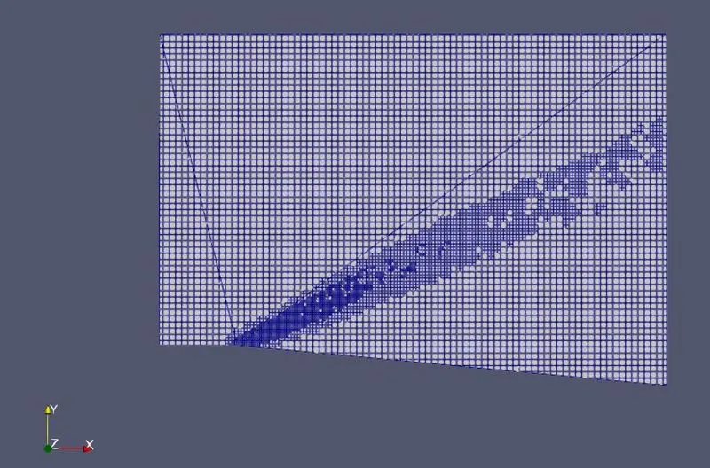
velocity contour-
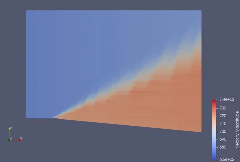
temperature contour-
pressure contour-
velocity plot at inlet-
velocity plot at outlet-
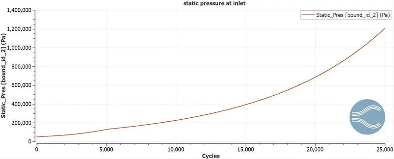
static pressure plot at inlet-
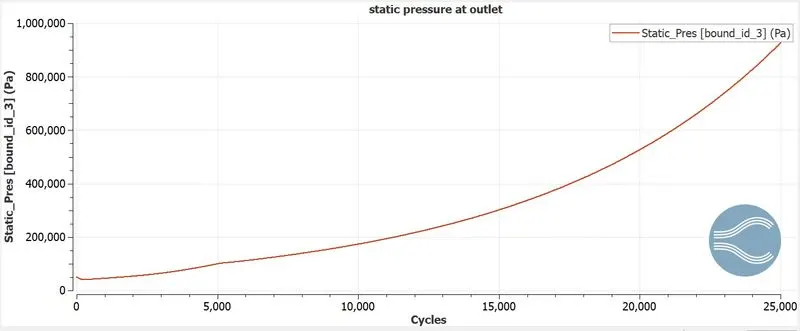
static pressure plot at outlet-
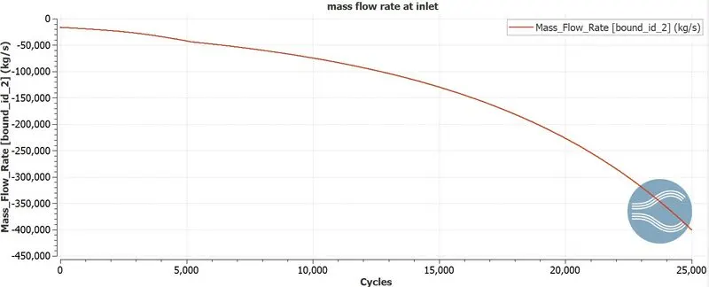
mass flow rate plot at inlet-
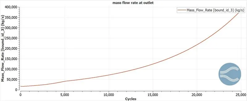
mass flow rate plot at outlet-
mach number plot at inlet-
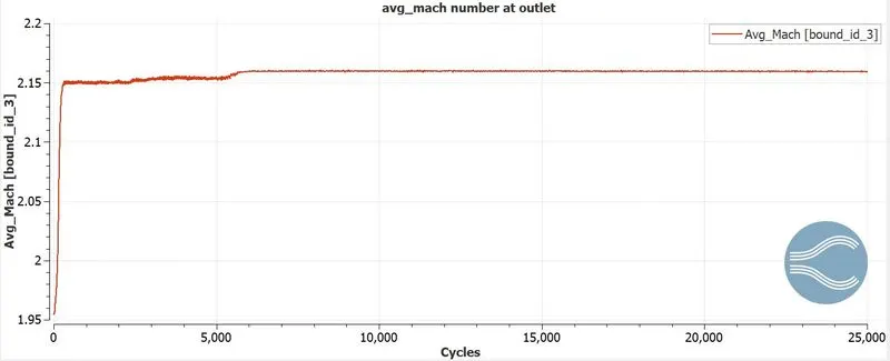
mach number plot at outlet-
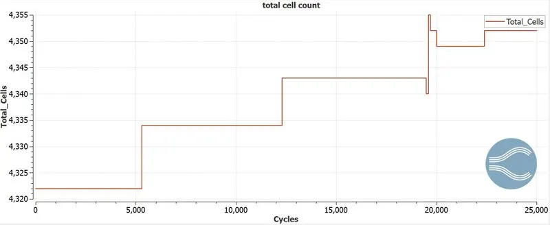
total cell count-
temperature animation of above simulation-
velocity animation of above simulation-
case b:
velocity 680 m/s and with SGS parameter 0.01 k
grid-
final grid after simulation-
velocity contour-
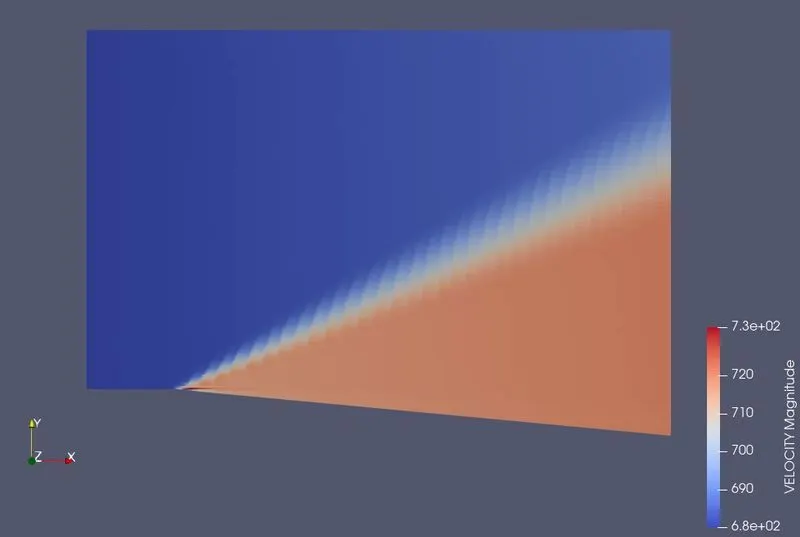
temperature contour-
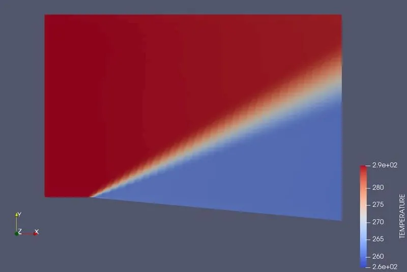
pressure contour-
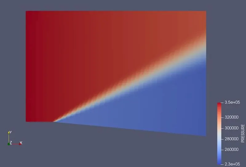
velocity plot at inlet-
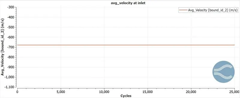
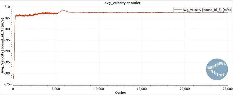
velocity plot at outlet-
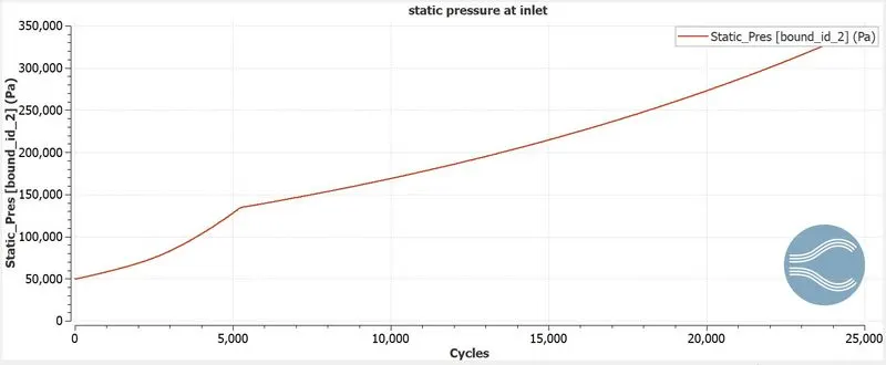
static pressure at inlet-
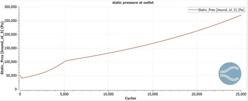
static pressure at outlet-
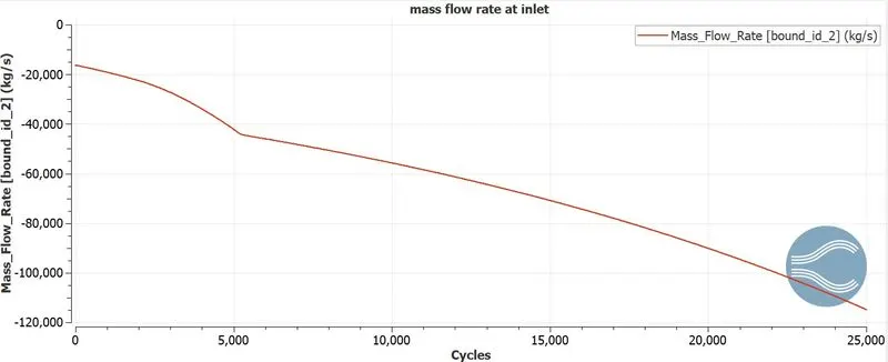
mass flow rate at inlet-
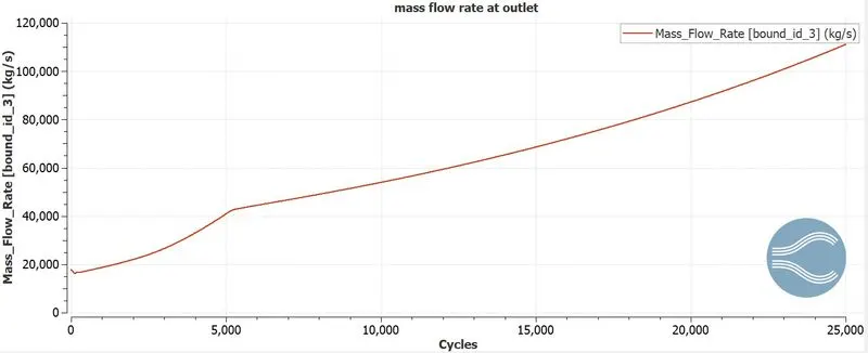
mass flow rate at outlet-
mach number plot at inlet-
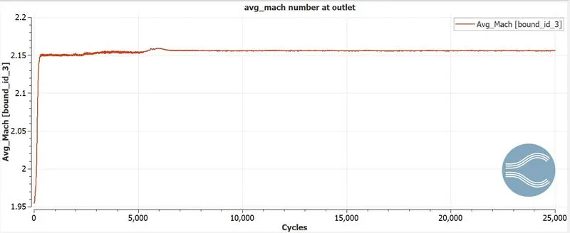
mach number plot at outlet-
total cell count-
temperature animation of above simulation-
velocity animation of above simulation-
case c:
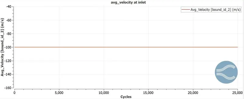
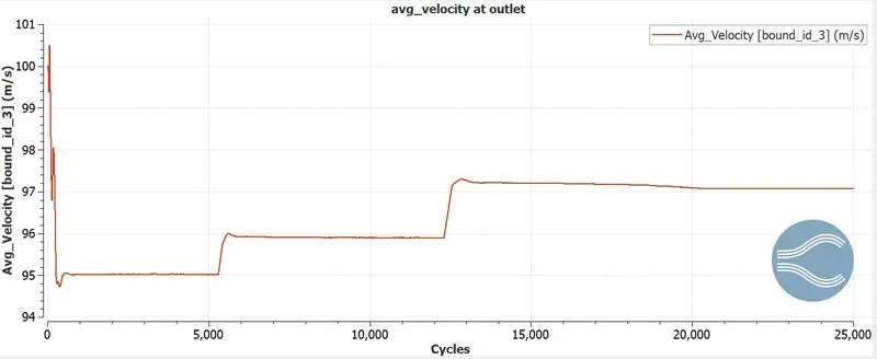
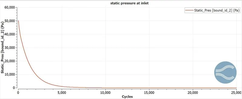
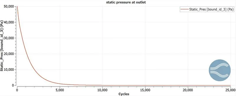
velocity 100 m/s and with SGS parameter 0.01 k
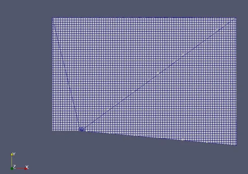
grid-
final grid after simulation-
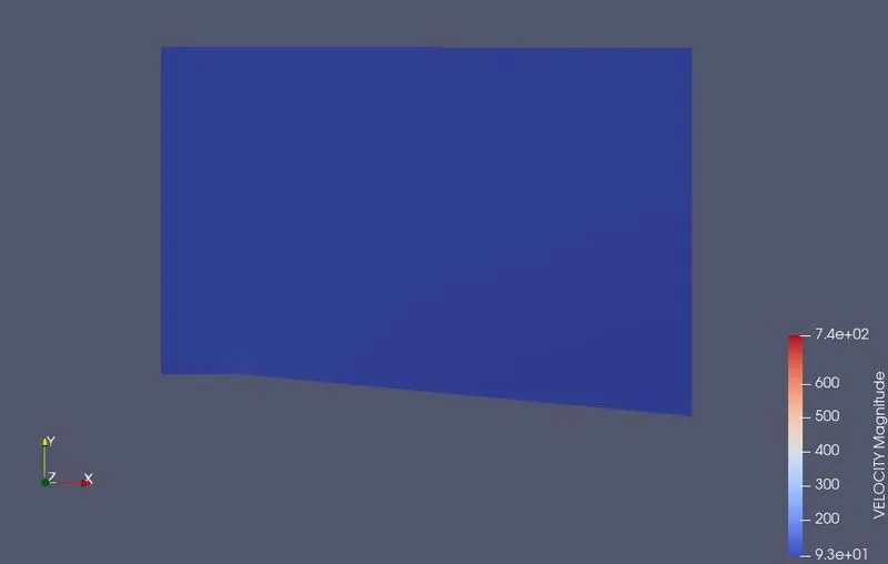
velocity contour-
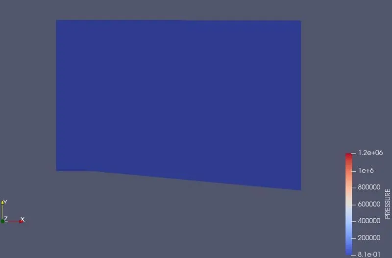
pressure contour-
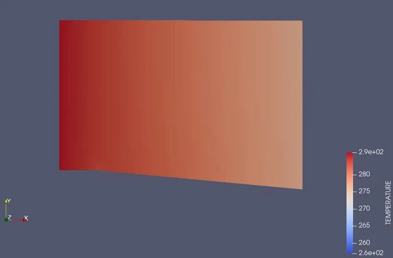
temperature contour-
velocity plot at inlet-
velocity plot at outlet-
static pressure plot at inlet-
static pressure plot at outlet-
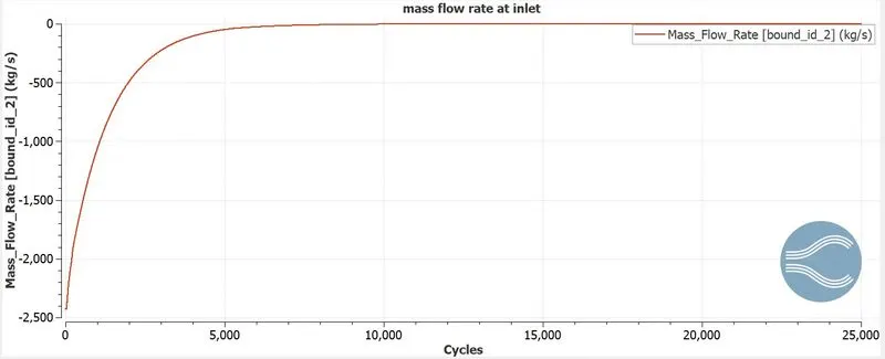
mass flow rate plot at inlet-
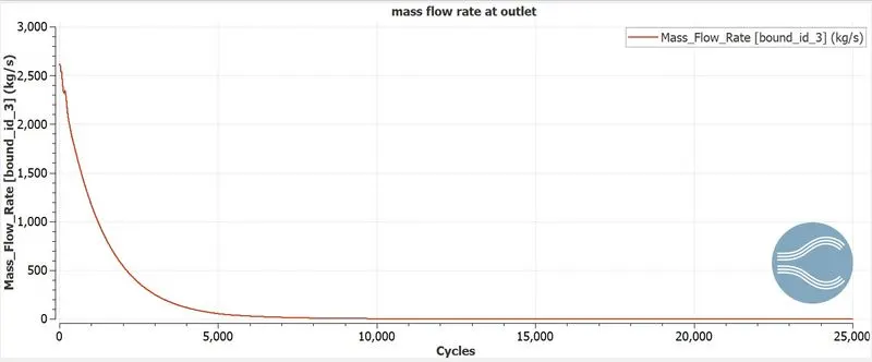
mass flow rate plot at outlet-
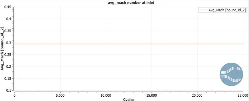
mach number plot at inlet-
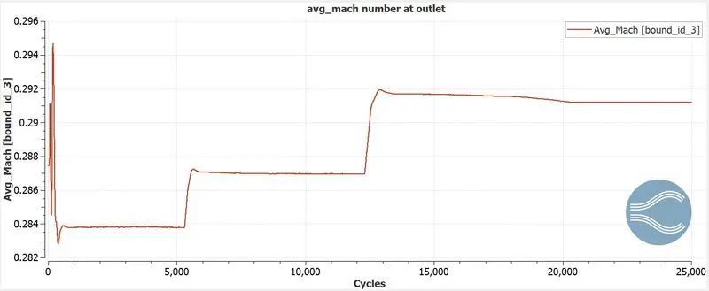
mach number plot at outlet-
total cell count-