Week 4.1 - Genetic Algorithm

Aim-Write a code in MATLAB to optimise the stalagmite function and find the global maxima of the function.

objective- To write a code in MATLAB to optimise the stalagmite function and find the global maxima of the function and Clearly expalin the concept of genetic algorithm in your own words and also explain the syntax for ga in MATLAB in your report.

BODY OF THE CONTANT:

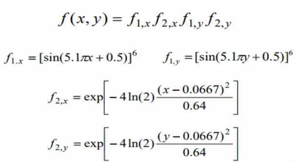
The above equations are used in the stalagmite function to plot the graph in the main functions.

function [f] = stalagmite(input_vector)

x = input_vector(1);

y = input_vector(2);

f1_x = (sin(5.1*pi*x + 0.5)).⁶;

f1_y = (sin(5.1*pi*y + 0.5)).⁶;

t1 = ((x-0.0667).²)/(0.64);

f2_x = exp(-4.*log(2)*t1);

t2 = ((y-0.0667).²)/(0.64);

f2_y = exp(-4.*log(2)*t2);

f = -(f1_x.*f2_x.*f1_y.*f2_y);

end

While using the function at the end as we are using the -ve sign so that the plot will be reversed as we have to find the maxima of the given function using ga.

Main body

• Firstly, creating the mesh from the two vectors which will be acting as a search space to find the maxima of the function.
• Creating the mesh of these two vectors using the ‘mesh’ command and defining the no. of iterations as num_cases to iterate the values of the optimum values of the function.
• Now calculating the values of fitness function at each point of the mesh grid formed.
• Now creating its surface through ‘surfc’ command which will also provide the contour of the generated surface.
• While using surfc applying the -ve sign to the function will generate the surface upside down which will be quite good to get the maxima of the function, as it will provide positive value for the maxima using the -ve sign.

clear all
close all
clc
%% PROVIDING THE SEARCH SPACE FOR THE FUNCTION
x=linspace(0,0.6,150);
y=linspace(0,0.6,150);
[X,Y]=meshgrid(x,y);
num_cases=50; %Number of itreation for which the function will evaluate the fitness
%% CREATING THE SURFACE PLOT OF STALAGEMITE FUNCTION
for i=1:length(X)
for j=1:length(Y)
input_vector(1)=X(i,j);
input_vector(2)=Y(i,j);
F(i,j)=stalagmite(input_vector); %values of function in given search space
end
end
surfc(X,Y,-f); %generating the surface
shading interp %To remove the lines produced by the mesh grid
%% STATISTICAL BEHAVIOUR (UNBOUNDED)
tic %calculating the study time through tic and toc command
for i=1:num_cases
[inputs,fopt(i)]=ga(@stalagmite,2); %calculating the optimized value of the function
xopt(i)=inputs(1); %at each iteration
yopt(i)=inputs(2);
end
study1_time=toc %displaying the time taken to evaluate
% PLOTING THE GRAPH
figure(1)
subplot(2,1,1)
surfc(X,Y,-f);
hold on
shading interp
plot3(xopt,yopt,-fopt,'marker’,’o’,’markersize’,5,’markerfacecolor’,’r');
xlabel('x');
ylabel('y');
grid on
subplot(2,1,2)
plot(-fopt);
xlabel('iterations')
ylabel('function min value')
%% STATISTICAL BEHAVIOUR (BOUNDED)
tic %calculating the study time through tic and toc command
for j=1:num_cases
[inputs,fopt(j)]=ga(@stalagmite,2,[],[],[],[],[0;0],[1;1]); %calculating the optimized value of the function
xopt(j)=inputs(1); %at each iteration with boundation
yopt(j)=inputs(2);
end
study2_time=toc
%PLOTTING
figure(2)
subplot(2,1,1)
hold on
surfc(X,Y,-f)
shading interp
plot3(xopt,yopt,-fopt,'marker),’o’,’markersize’,5,’markerfacecolor’,’r');
xlabel('x');
ylabel('y');
grid on
subplot(2,1,2)
plot(-fopt);
xlabel('iterations')
ylabel('function min value')
%% MODIFYING THE NUMBER OF POPULATION
options=optimoptions('ga’,’populationsize',300) %increaing the sixe of population by using
%optimoptions function
tic
for k=1:num_cases
[inputs,fopt(k)]=ga(@stalagmite,2,[],[],[],[],[0;0],[1;1],[],[],options);
xopt(k)=inputs(1);
yopt(k)=inputs(2);
end
study3_time=toc
%PLOTTING
figure(3)
subplot(2,1,1)
hold on
surfc(X,Y,-f)
shading interp
plot3(xopt,yopt,-fopt,'marker’,’o’,’markersize’,5,’markerfacecolor’,’r');
xlabel('x');
ylabel('y');
grid on
subplot(2,1,2)
plot(-fopt);
xlabel('iterations')
ylabel('function min value')