Week 5: Prandtl Meyer Shock problem
Introduction :
In 1907, German fluid dynamicist Ludwig Prandtl studied the expansion waves, followed by his student Theodor Meyer in 1908. They developed a theory called Prandtl Meyer expansion to explain the behavior of expansion wave.
A Supersonic expansion fan, technically known as Prandtl-Meyer expansion fan, a two-dimensional simple wave , is a centered expansion process that occurs when a supersonic flow turns around a convex mirror. The fan consist of an infinite number of Mach wave, diverging from a sharp corner. when a flows turns around a smooth and circular corner, these waves can be extended backwards to meet at a point.
1. Shock flow boundary conditions?
Both ordinary and partically differential equations need boundary conditions to be solved. Different type of boundary conditions can be imposed on the boundary of the domain. The choice of the boundary condition is fundamental for the resolution of the computational problem a bad imposition of b.c lead to the divergence of the solution or to the convergence to a wrong solution.
Types of Boundary conditions are as follows:
Dirichlet boundary condition: When the boundary condition is imposed on ODE or PDE its specifies the value of the function or variable at the boundary.
Neumann boundary condition: When the boundary condition is imposed on ODE or PDE the condition specifies the value in which the derivative of the solution is applied within the boundary of the domain.
Robin BC : This condition when imposed on ODE or PDE , it specifies the values of the field and its derivative of the boundary , this condition is also known as impedance condition.
Cauchy BC : It is the condition on both the unknown field and its derivative. It differs from Robin condition because it implies the imposition of two constraints while robin condition implies only one constraint on the linear combination of unknown function and its derivative .
Boundary Condition used in Shock Flow –
Neumann Boundary condition are preferred over other in shock flow as thermodynamic properties can oscillates and values had to be extrapolated from the interior regions at each states rather than providing specifics values which could deaccelerate the convergence of solution.
2. What is Shock wave?
A shock wave is type of propagating disturbance that moves faster than the local speed of sound in the medium. Like an ordinary wave,a shock wave carries energy and can propagate through a medium but is characterized by an aburpt, nearly discountinous,change in pressure,temperature and density of the medium.
Shocks are of 2 types:
- Normal Shock - Shock created at 90 degrees.
- Oblique Shock - Shock created at an angle as per the body\'s deflection angle.
Why Neumann boundary condition used for supersonic outlets?
For a supersonic outlet, the characteristic curves propagate outside the domain, along with the streamline. Hence the values of the variable need to be floated, i.e. we calculate the values using linear extrapolation. Hence, we have used Zero normal gradient as the boundary condition for pressure and velocity.
Procedure :
1. Provided geometry is dropped in the Converge workspace.
2. Boundaries are named using appropriate names.
3. Normal direction are checked to be in line with the geometry and flow.
4. Diagnosis is performed to check any discrepancies in geometry.
5. Then appropriate species are selected for the fluid.
6. Simulation parameters along with the steady-state monitor are set.
7. Boundary conditions are set to the appropriate regions and their corrosponding values.
8. The base grid of the considered step size is inserted along with respective directions and associated temperatures AMR with the desired SGS value.
9. Variables for post-processing and time intervals for writing the output and restart files are set and selected.
10. All the input files are stored at the desired location.
11. All the stored input files are executed using the command editor. These input files are executed by Converge Solver in the background.
12. Then the executed files generated the output folder in which data files after every selected cycle intervals are stored which are post processing for the graphical results.
## There is a slight change in the boundary condition which explained below:[ GIven hint to
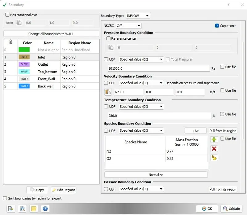
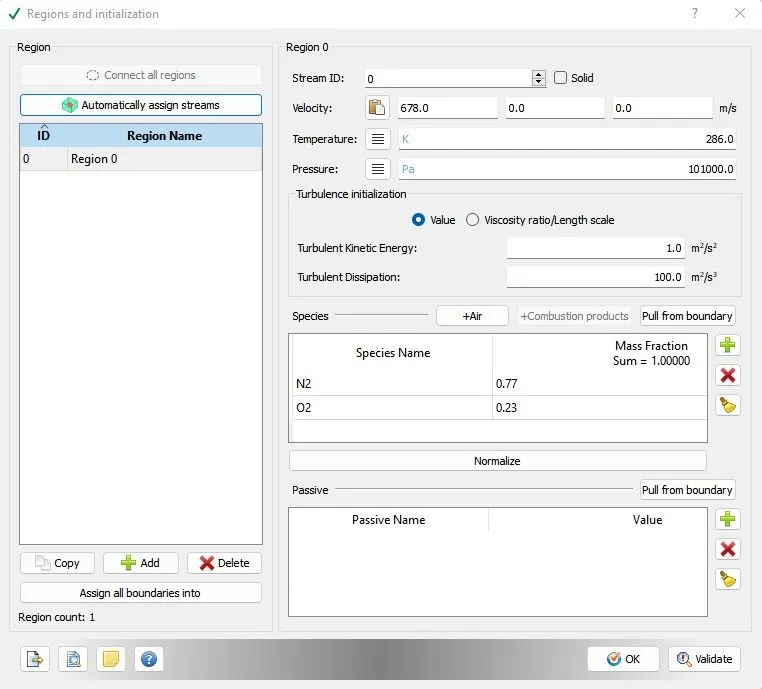
Inlet: Since it’s a supersonic flow at the inlet we should assign Dirichlet boundary conditions for all parameters like Pressure, Velocity, and Temperature. So, We can give Static pressure= 101000 Pa, Velocity=678m/s and Temperature=286k
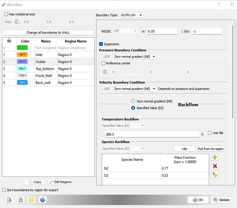
Outlet: At the outlet, we should assign Neumann boundary conditions for all parameters like Pressure, Velocity, and Temperature. So, We can give a Zero normal gradient for all the parameters.
Top-Bottom wall:
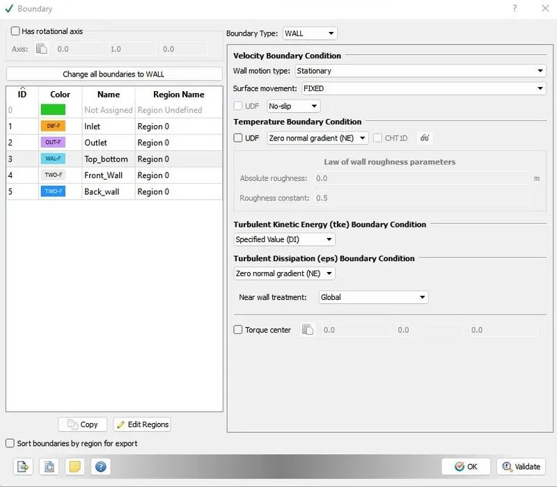
Since the supersonic flow is inviscid in nature(the viscous effect is negligible) we can assume the Slip condition at the wall.
Front-Back: 2D Wall Reason: The 2D planar assumption is used because the flow gradients along the z-direction are negligible when compared to the other two directions. By reducing the model to 2D, the Prandtl Meyer can be simulated and analyzed cost-effectively compared to a full 3D model.
Turbulence Modelling: No need for the Turbulence model.
Reason: In our simulation, we don't have to use Turbulence modeling since there is no Reynolds stress because the flow is inviscid.
PROCEDURE:
The geometry is imported and the boundary flagging is done.
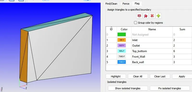
Once the boundaries are alloted then we proceed for the case setup.
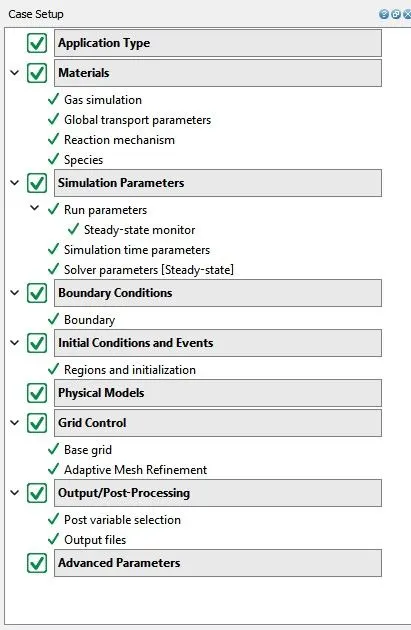
Run Parameters :-
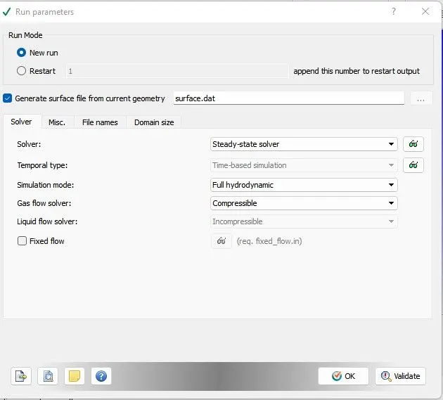
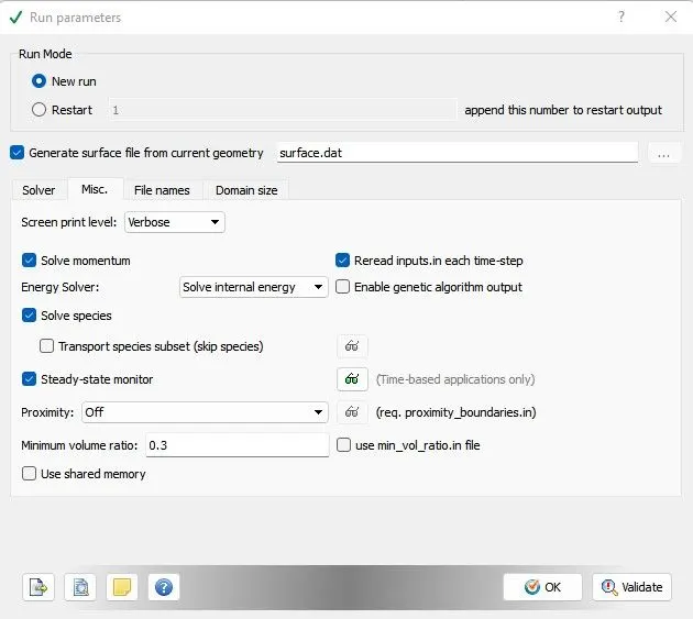
Steady-State Monitor :-
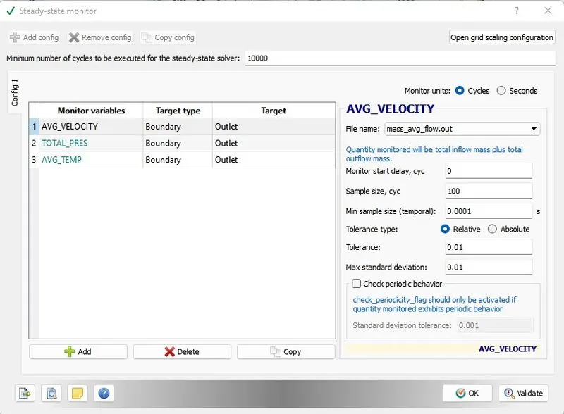
Minimum no. of cycle = 10000
Sample size = 100
so by this i will going to get max. time step in PARAVIEW = 100
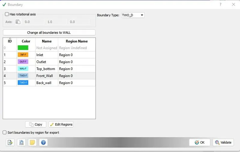
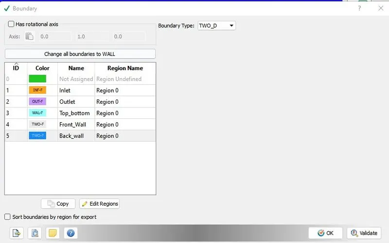
Boundary Conditions :-
Inlet :
Velocity = 678 m/s in x direction
Temperature = 286 k
Exit :
Pressure - Zero normal gradient
Velocity - Zero normal gradient
Front and Back - 2D
Top and Bottom Wall - Slip Wall
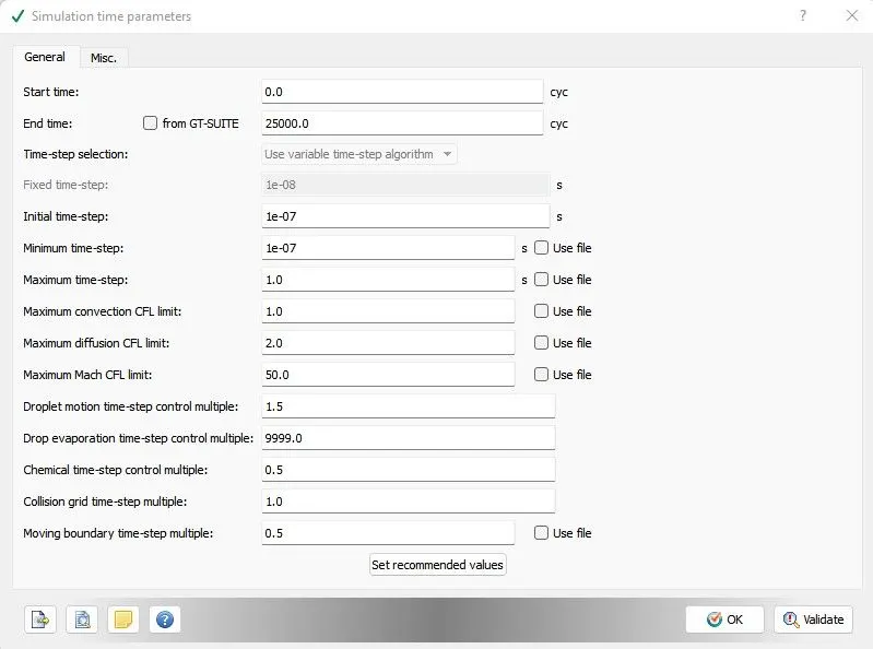
Simulation Time Parameters :
Start Time : 0 Cycle
End Time : 25000 Cycle
Solver : Density based Steady state solver
Fluid under Consideration : Air (O2 + N2)
CFL = 1
Region and Initialization :
Adaptive mesh Refinement :-
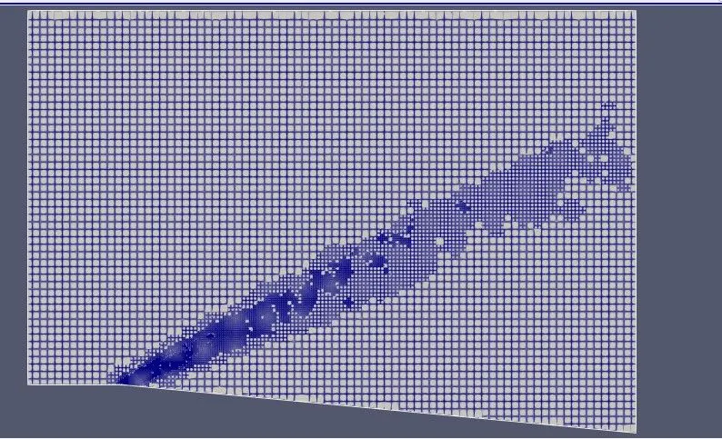
Mesh size of 0.8 m was provided in X, Y, Z directions along with adaptive mesh refinement.
Temperature AMR was provided with maximum embedding level of 2 and sub-grid scale criteria as 0.05.
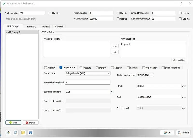
Sub-grid scale is a parameter which will be used by converge for refining the mesh. Converge monitors the curvature of the fluid property provided in the AMR and refines the mesh when the property curvature variation between the consecutive grid is more than the defined SGS value.
Base Grid :
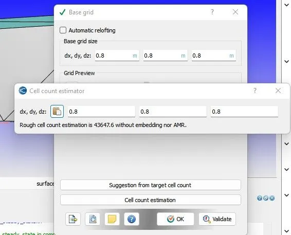
Grid size of 0.8m is used and adaptive mesh refinement is also done to the geometry.
Output files :-
Output data files = 125
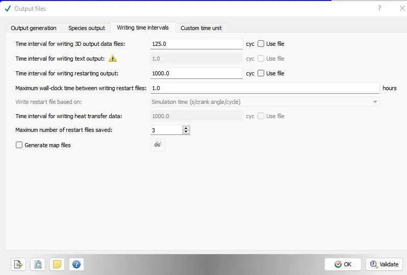
After the Case Setup export the files to destination folder(week 5) and copy the file such as converge and mpiexe from the Converge installation folder and paste it into the week 5 folder and then GO to CYGWIN and Run the simulation by a given command
mpiexec.exe -n 3 converge.exe restricted
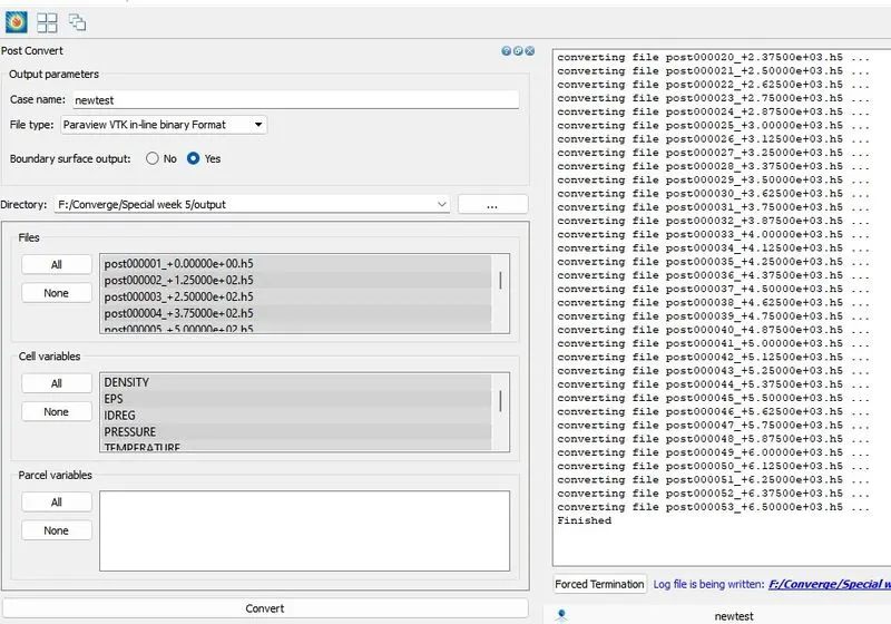
After this Go to Converge --- > POST CONVERT --> Upload the file --> destination folder -- > Output -- > Apply and Run the post process Here.
Choose File type here as Paraview VTK in-binary Format
and select the ALL Button from Files, Cell Variables, Parcel Variabes and Hit on Convert button.
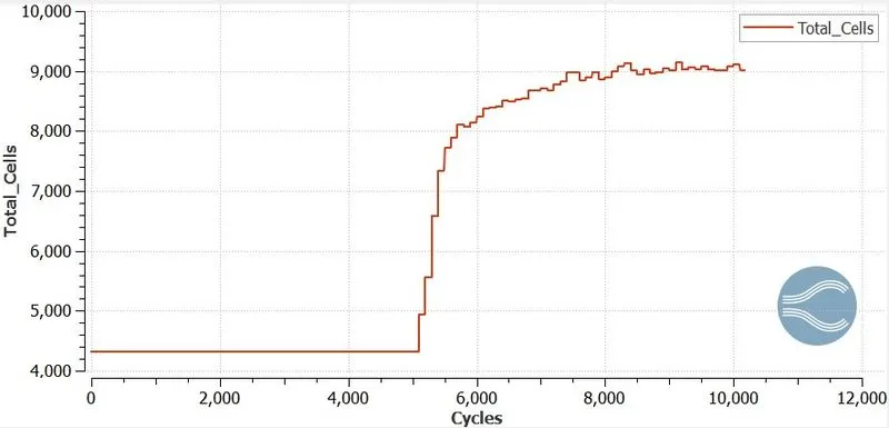
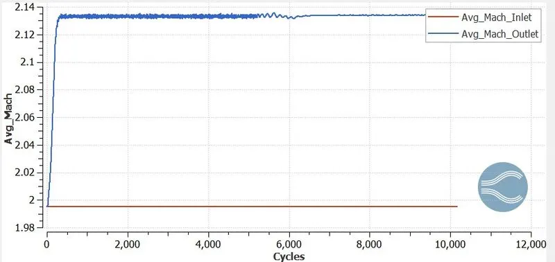
Next, move to Line plotting and upload the destination file here and make total cells and mach number plots here.
Case : Inlet Velocity = 678m/s (Supersonic flow) and Subgrid criterion (SGS) parameter = 0.05
PLOTS:-
Total Cells
Mach Number
The next setp is to plot the contours and make the animation so for this Let's go to
PARAVIEW and upload the file from the extention .vtm which was formed during the post processing whatever the name we give on that time in te Case name ____
upload it.
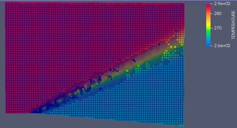
RESULTS :- The results below describe the variation of parameters over the simulation with the SGS of 0.05.
Mesh Contour
Temperature Contour
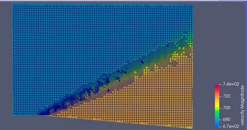
Velocity Contour
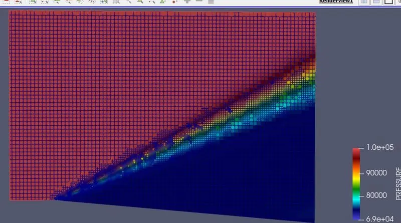
Pressure Contour
ANIMATION :-
Temperature Animation
Pressure Animation
Velocity Animation
Google drive link
https://drive.google.com/file/d/1B3EVKGaeYw9UrGS_4jJpNWKedbMe_OSB/view?usp=sharing
NOTE : - When i am going to take SGC = 0.5 with velocities 100m/s and 678 m/s then i got wrong profils in the PARAVIEW.
Subsonic Vs Supersonic Flow Comparison
In supersonic flow, the Prandtl-Meyer expansion fan is clearly visible and the mesh refinement is also visible in the shock region
Whereas on the other hand, in the case of a subsonic flow, the Prandtl-Meyer expansion fan is not at all visible and even the mesh refinement is not visible. This is because there are no sudden fluctuations in pressure, velocity, temperature, or density, or in other words, shock.
Also, the average Mach number increases from the inlet to the outlet in case of supersonic flow and decreases in case of subsonic flow.
3. Effect of SGS parameter on shock location.
Conclusion :-
1. Prandtl-Meyer Expansion Fan only works with supersonic streams not sub sonic as velocity of 2 Mach shows the phenomena but not with 100 m/sec.
2. The pressure, temperature, density decrease across the Mach waves, however the velocity increases, for the supersonic inlet.
3. As SGS decreases the accuracy of the solution increases and calculation time also increases.
4. SGS 0.05 gives the best result of 2.153 Mach Number at outlet boundary
5. Number of cells increase with decrease in SGS parameter as refinement becomes more sensitive with lower SGS.
5. The 0.5 Temperature Sub-grid-scale criteria isn't able to capture the Mach wave properly hence the pressure value does not decrease as much as it should.
Results :
Studied the behaviour of flow variables (velocity, Temperature, Pressure, denisty and Mach number) when the fluid flow past the sharp corner in the geometry.
For supersonic inlet velocity, the Variables Velocity and Mach number increases past the corner till the outlet and all other variables reduces so there by maintaining the constant total pressure. The behaviour is opposite for the subsonic inlet here velocity reduces and other variables increase past the corner.
For supersonic inlet, we can say the expansion process takes place past the corner producing the shock waves at some angle to the horizontal across which the velocity of the fluid increases increasing the mach number and reducing pressure, density and temperature.Total pressure remains constant in the system. Studied the production of Shock waves for supersonic inlets.
Lower the value of the Temperature SGS, the higher the cell number, making the mesh finer in large area thereby the capturing the values accurately and increasing the simulation time.