Week 5: Prandtl Meyer Shock problem

AIM:

• To simulate a Prandtl Meyer wave. The location and nature of the shock formed are examined. Also, the impacts of adaptive Mesh refinement are studied.

THEORY:

SHOCK WAVES:

• Shock waves are essentially non-linear waves that propagate at supersonic speeds. They can be visualized as a very sharp and thin wavefront across which pressure, temperature, density, entropy and velocity of flow change abruptly.
• This means that the region between the body and the shock wave usually referred to as the shock layer will be a region of high pressure, temperature and density compared to the free stream flow conditions.
• This sudden change in the medium of propagation is one of the unique features that characterize the shock wave. Due to the sudden changes in flow properties, shock waves are often regarded as discontinuities with highly localised irreversibiliities.
• The typical thickness of the shock in standard atmospheric air is about 2.5 Angstrom, very small compared to other characteristic lengths in fluid flow.

Types of Shock Waves:

1. Moving Shock- Consists of a shock propagating into a stationary medium

2. Detonation Wave- A detonation wave is essentially a shock supported by a trailing exothermic reaction. It involves a wave travelling through a highly combustible or chemically unstable medium, such as an oxygen-methane mixture or a high explosive. The chemical reaction of the medium occurs following the shock wave, and the chemical energy of the reaction drives the wave forward.

3. Bow Shock- These shocks are curved and form a small distance in front of the body. Directly in front of the body, they stand at 90 degrees to the oncoming flow and then curve around the body.

4. Attached Shock-These shocks appear as attached to the tip of sharp bodies moving at supersonic speed.

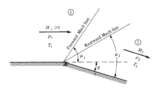
• An expansion fan, sometimes called a Prandtl-Meyer expansion wave, is considered a continuous sequence of infinitesimal Mach expansion waves. It is a 2D simple wave that occurs when a supersonic flow turns around a convex corner. Some qualitative aspects of flow through expansion waves are given below

1. An expansion corner is a means to increase the flow Mach Number.

2. The pressure, temperature and density decrease through an expansion wave.

3. Streamlines through an expansion wave are smooth curved lines

4. Since the expansion takes place through a continuous succession of Mach waves and ds=0, for each Mach wave the expansion is isentropic.

A. CASE SETUP:

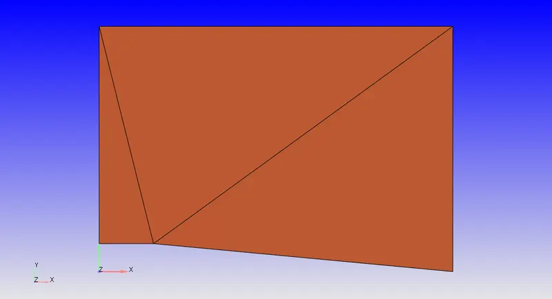
1. Geometry Creation:- The geometry in STL format was imported into CONVERGE for analysis.

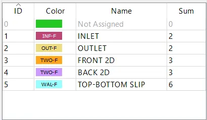
2. Creation of Boundaries: In the geometry which is created above, boundaries such as inflow, outflow, top and bottom walls, and front and back faces are labelled.

3. Checking Orientation of Normals: Orientation of Normals was checked to ensure all the normals are pointing inwards. This was done using the Normal Toggle

4. Finally a Diagnosis check was run to ensure no errors in the geometry.

B. CASE SETUP:

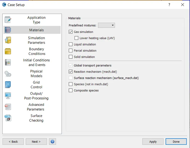
1. Application Type:- This was set to Time based,

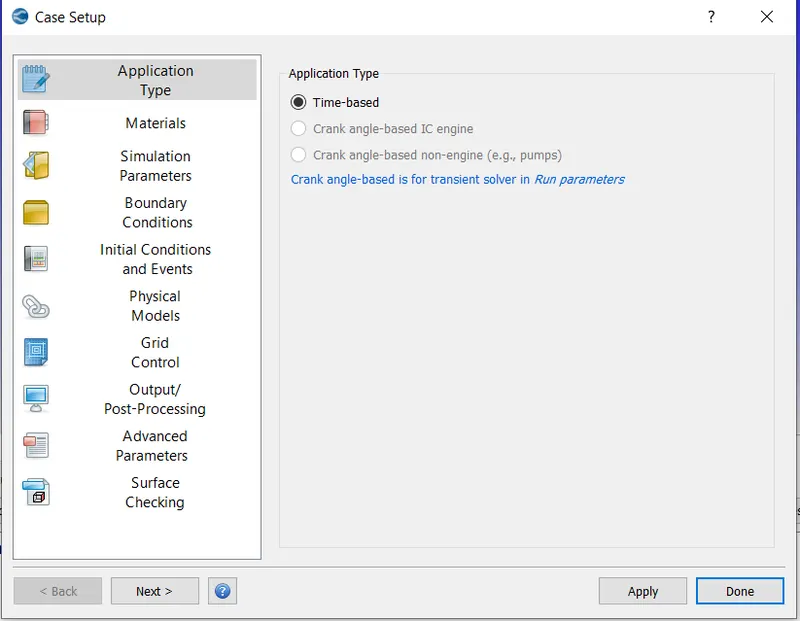
2. Materials:- This was set to Air,

1. Gas Simulation: Default properties were retained,
2. Global Transport Parameters:- Default properties retained.

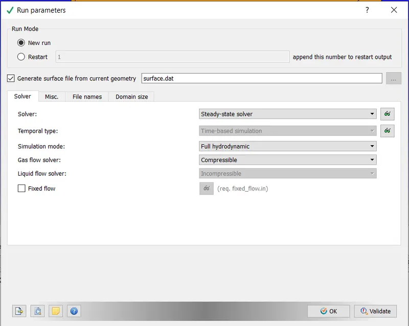
1. Simulation Parameters:

- Run Parameters:- Steady state solver was used. The simulation mode was set to Full Hydrodynamic. The gas flow solver is set to Compressible,

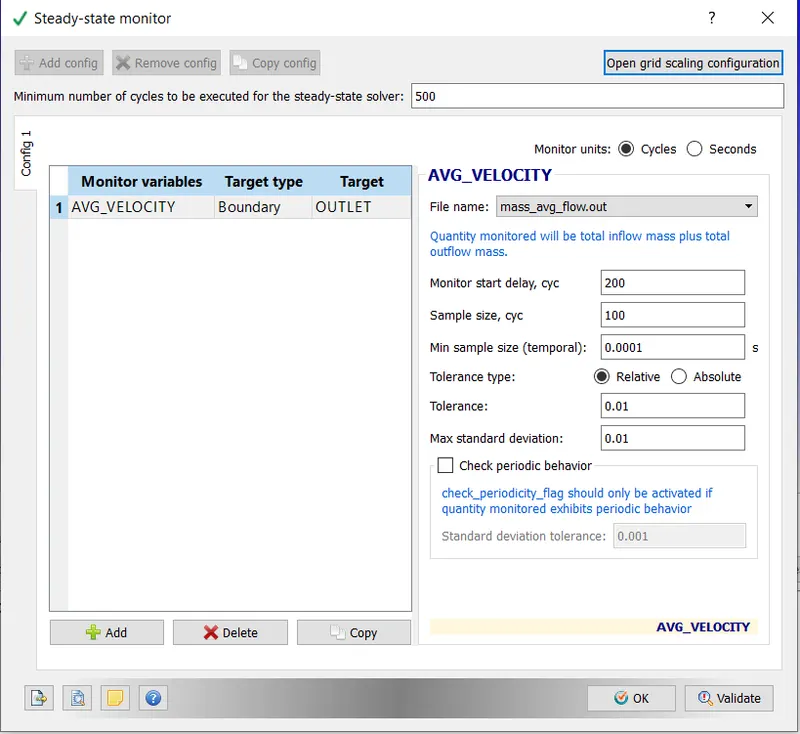
- Steady State Monitor:- Minimum no of cycles to be executed for Steady-state solver -500

Monitor Start Delay, cyc:- 200

Sample size cyc:- 100

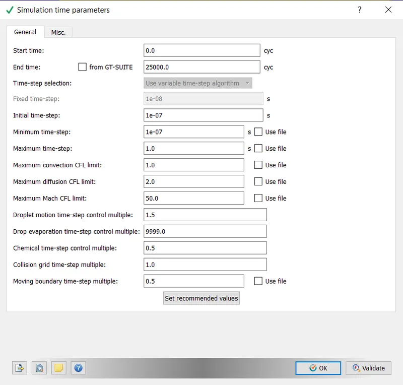
- Simulation Time Parameters:- The parameters were set as displayed below. The simulation was run for 25000 cycles. Max CFL limit set to 1.0

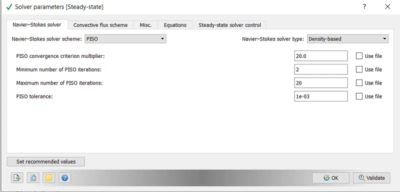
- Solver Parameters:- A Pressure based PISO solver was used, Maximum Convection CFL limit was set to 0.8.

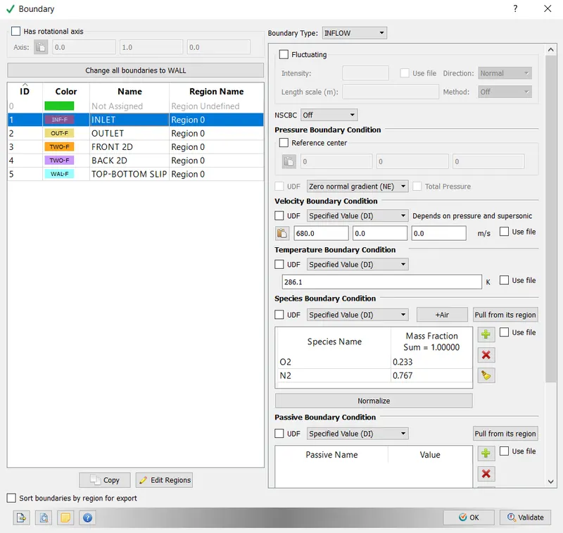
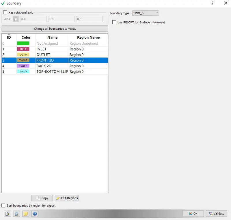
4. Boundary

- Inlet:- Boundary flow - Inflow

Inlet Velocity:- 680 m/s (Supersonic)

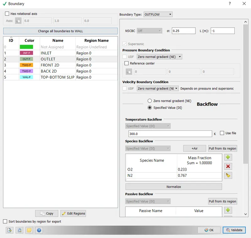
- Outlet- Boundary - Outflow with zero normal gradients for both Pressure and Velocity Boundary condition. We use a Neumann boundary condition since at the supersonic boundary condition it is not possible to predict the flow properties.

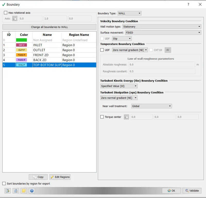
- Top and Bottom Walls:- Stationary wall with Fixed surface movement with slip boundary condition is used

- Front and Back faces set to Two D,

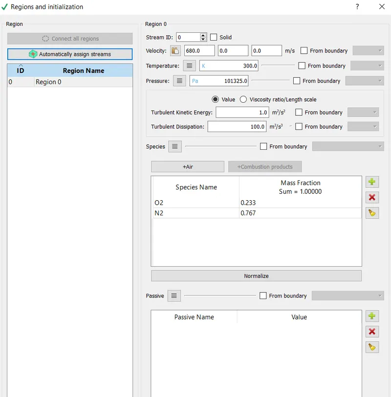
4. Initial condition and events

The created geometry was selected as the Volumetric Region. The velocity was set to 680m/s,

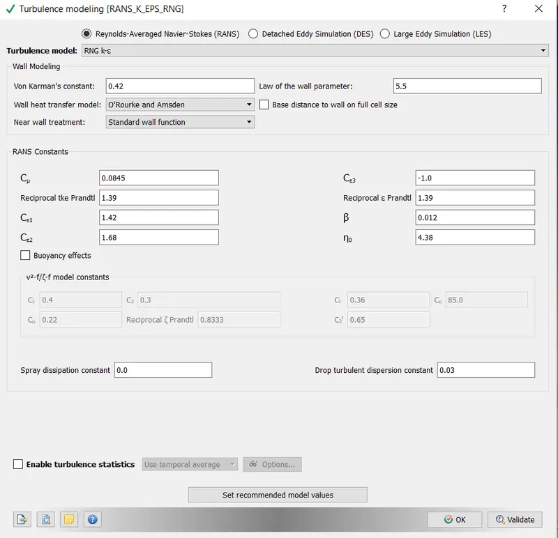
5. Physical Models:- RNG k epsilon used,

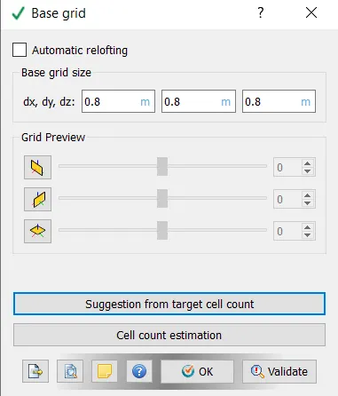
5. Grid Control:- Base Grid. Here the size of the mesh is entered.

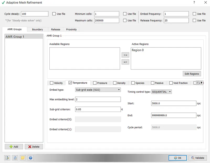
• Adaptive Mesh Refinement was also enabled. A temperature-based adaptive mesh,

• Whenever the curvature of temperature is greater than a particular value the mesh would be refined. It can be thought of as a sub-grid scale temperature.

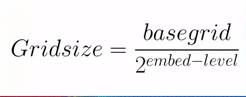
• In the below snapshot, we see that the sub-grid scale criterion is set to 0.05K. This implies that whenever the temperature difference is greater than 0.05 K, AMR will refine. The maximum embedding level is set to 2, this means that there will be two layers of refinement. Converge uses an octree data structure. In this data structure, the grid size can be calculated by the given formula

• In this case, the base grid size is 0.08. The smallest grid size will be 0.08/(2^2) which means the smallest grid size will be 0.02.

7. Output/Post Processing:- The variables that we intend to see during post-processing are selected. In this case, Density, Pressure, Temperature and Velocity were selected. Also, the frequency of generation of output files was set below, After setting the above, the input files were exported to a directory.

RESULTS:

CASE-1:

• Velocity-680m/s,SGS=0.05K,

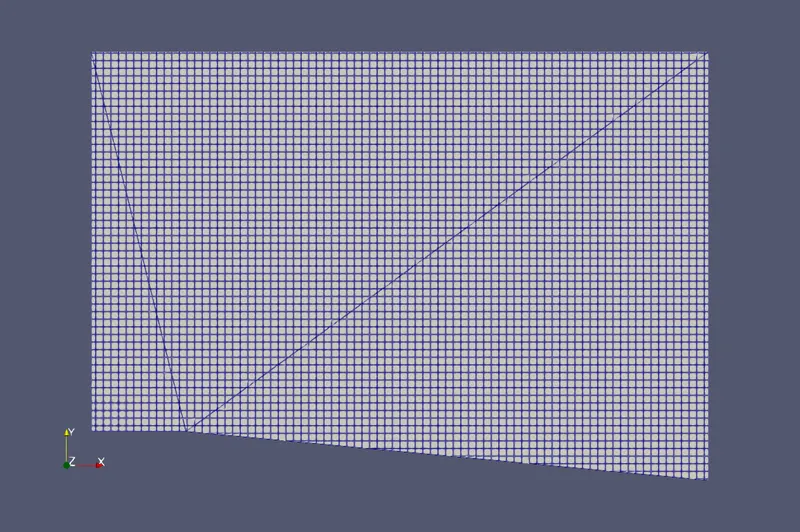
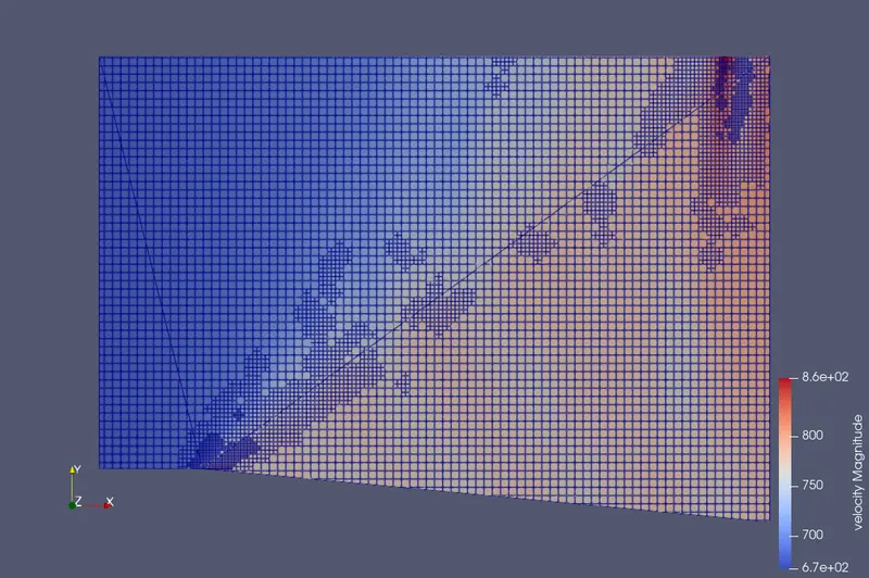
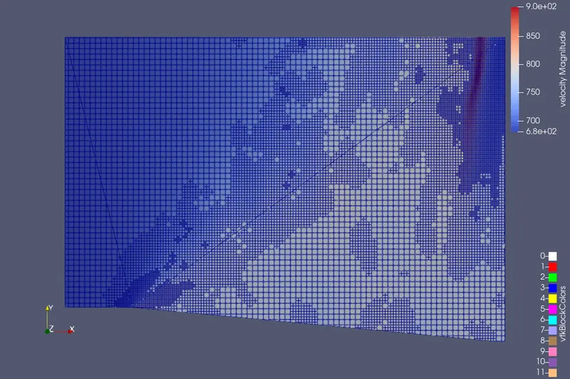
• Meshing:- The refined areas are those where the temp difference is greater than 0.05K,

• MESH VIEW:

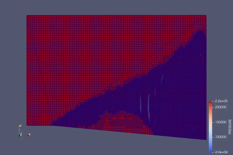
• PRESSURE CONTOUR:

• VELOCITY CONTOUR:

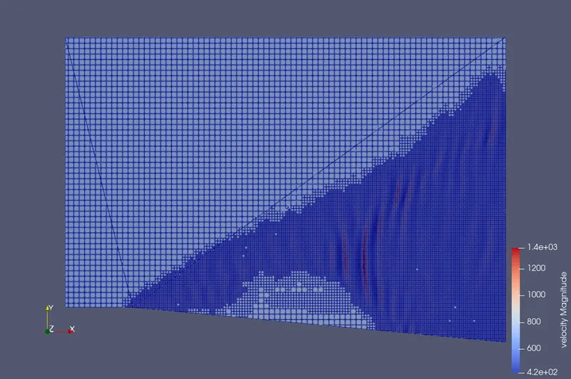
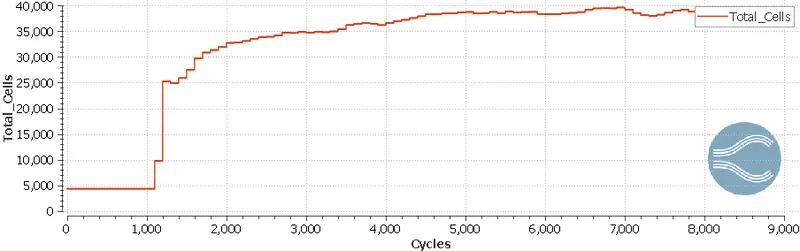
• CELL COUNT:

• VELOCITY ANIMATION:

CASE-2:

• Velocity-680m/s,SGS=0.03K,

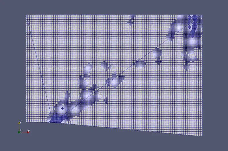
• Meshing:- The refined areas are those where the temp difference is greater than 0.05K,

• MESH VIEW:

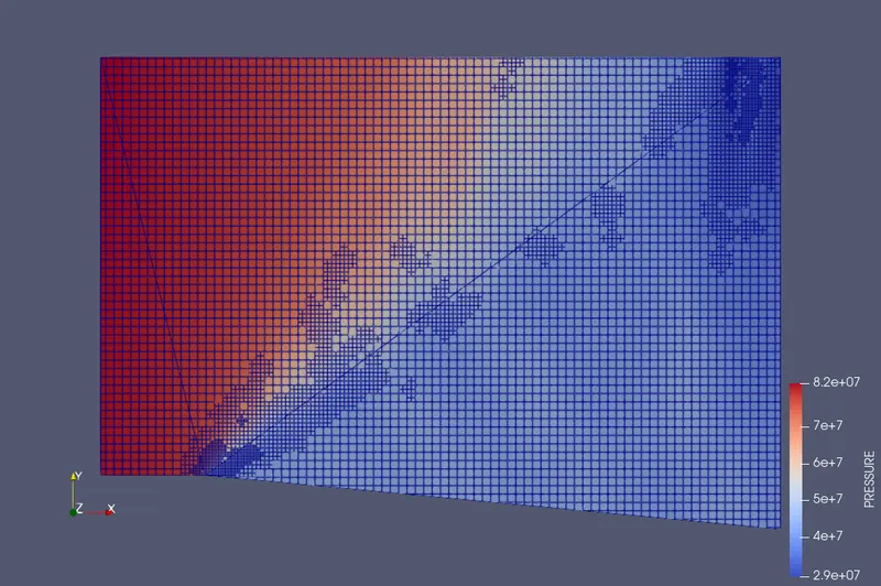
• PRESSURE CONTOUR:

• VELOCITY CONTOUR:

• CELL COUNT:

• VELOCITY ANIMATION:

CASE-3:

• Velocity-680m/s,SGS=0.01K,

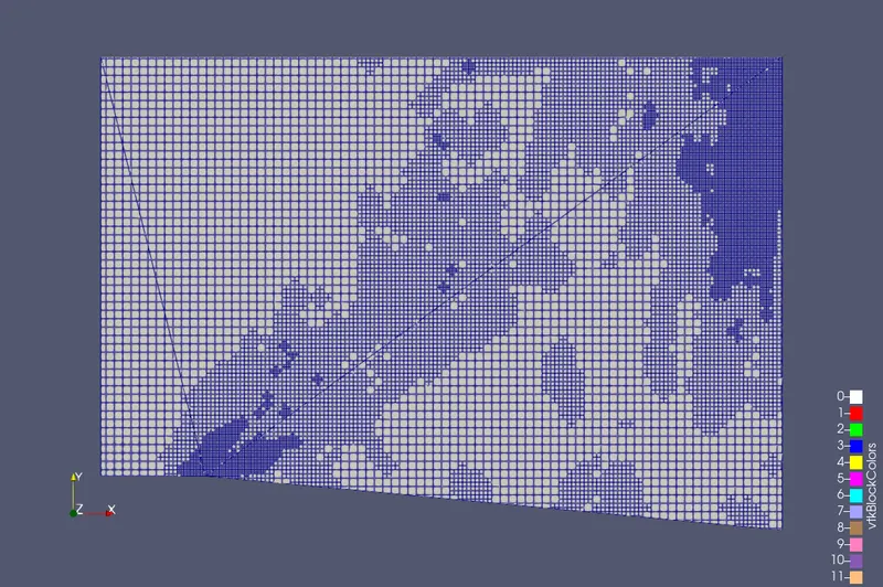
• Meshing:- The refined areas are those where the temp difference is greater than 0.05K,

• MESH VIEW:

• PRESSURE CONTOUR:

• VELOCITY CONTOUR:

• CELL COUNT:

• VELOCITY ANIMATION:

CONCLUSION:

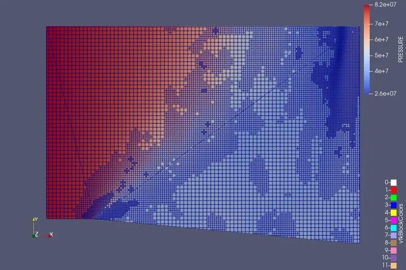
• Across the expansion wave, velocity and Mach number increase, whereas pressure, density and temperature decrease from inlet to outlet.

• With the decrease in SGS factor from 0.05 K to 0.01 K, we note the variation of properties such as velocity, and pressure. Mach Number and density can be observed more clearly.

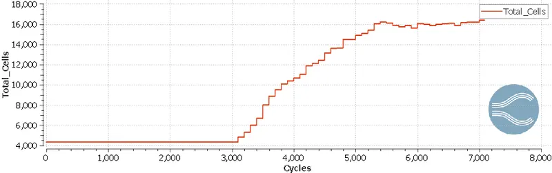
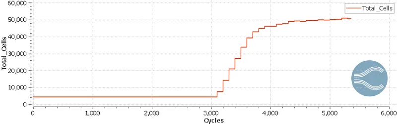
• There is an increase in the number of cells when the sub-grid scale factor is 0.05K to 0.01K. Also, the area of the Adaptive mesh refinement region increases with a reduction in SGS value.

• The location of the expansion waves shifts slightly rightwards with the reduction of the SGS value.