Week 5 - Mid term project - Solving the steady and unsteady 2D heat conduction problem

Aim: Solving 2-D heat conduction equation (steady and unsteady)

Objective:

• Solving the steady and unsteady state heat conduction equation by forming iterative solvers of
  
  • Jacobi
  • Gauss-Siedel
  • Succesive over relaxation (SOR)
• The solvers are provided with a relaxation factor, and appropriate boundary condition; Thus evaluate the most effective iterator by generating plots and the number of iterations required to obtain the same.
• Apply implicit and explicit schemes for transient analysis and compare the results.

Theory:

The 2-D heat conduction equation is given as:

`(delT)/(delt) = alpha[(del^2T)/(delx^2) + (del^2T)/(dely^2)]`

The equation is a partial differential equation which governs heat transfer through a conduction in 2-D reference frame. `alpha` is the thermal diffusivity which is characteristic for a medium.

In our solution, we are provided with a square domain of length equals to unity. This domain would be divided into smaller elements to implement discretization schemes. We are also provided with the boundary conditions to obtain a specific solution to this problem. The boundary conditions are defined as:

• Left boundary: `T(x=0,y) = 400K`
• Bottom boudary: `T(x,y=0) = 900K`
• Right boundary: `T(x=L,y) = 800K`
• Top boundary: `T(x,y=L) = 600K`

The equations for steady and transient states are solved separately.

Steady-State:

The time derivative vanishes in steady state and the equation reduces to,

`(del^2T)/(delx^2) + (del^2T)/(dely^2) = 0`

The above equation is disretized by central differencing scheme in both `x` and `y` directions, hence,

`(T_{i-1,j} - 2T_{i,j} + T_{i+1,j})/(Deltax^2) + (T_{i,j-1} - 2T_{i,j} + T_{i,j+1})/(Deltay^2)`

As we are assuming `nx = ny`, thus, `Deltax = Deltay = h`. Hence, we have,

`T_{i,j} = (T_{i-1,j} + T_{i+1,j} + T_{i,j-1} + T_{i,j+1})/4`

This is the final equation that is solved using Jacobi, Gauss-Siedel and SOR methods.In Jacobi method, the values are taken from the old iteration, in Gauss-Siedel, the values get updated within the iteration and SOR is improved Gauss-Siedel, where values are updaetd as per the relaxation parameter.

Transient-State (Explicit):

In transient state the time derivative exists, hence, we use the complete heat conduction equation. Discretization is done by forward differencing scheme. The sheme can be explicit or implicit depending on the time-step at which the spatial derivatives are chosen. Thus the equation on discretization becomes:

`(T_{i,j}^(n+1) - T_{i,j}^n)/(Deltat) = alpha[(T_{i-1,j} - 2T_{i,j} + T_{i+1,j})/(Deltax^2) + (T_{i,j-1} - 2T_{i,j} + T_{i,j+1})/(Deltay^2)]`

Since, `Deltax = Deltay = h`

`T_{i,j}^(n+1) = T_{i,j}^n + (alphaDeltat)/h^2(T_{i-1,j}^n + T_{i+1,j}^n + T_{i,j-1}^n + T_{i,j+1}^n - 4T_{i,j}^n)`

`T_{i,j}^(n+1) = (1 - (4alphaDeltat)/h^2)T_{i,j}^n + (alphaDeltat)/h^2(T_{i-1,j}^n + T_{i+1,j}^n + T_{i,j-1}^n + T_{i,j+1}^n)`

where, the superscript `n` denotes the time-step.

For stability, the term of `T_{i,j}^n` in the RHS cannot be negative. This results in Courant-Friedrich-Lewy (CFL) condition for stability. The term `(4alphaDeltat)/h^2` is the CFL number. Hence, we can calculate the maximum time-step that can be chosen for explicit method.

`1 - (4alphaDeltat)/h^2 >= 0`

`:. Deltat <= h^2/(4a)`

Hence, the abve condidtion must also be kept in consideration while solving by explicit solver.

Transient-State (Implicit):

For the implicit solver,. the `T` terms are taken at `n+1` instead of `n`. Thus the equation changes to

`T_{i,j}^(n+1) = T_{i,j}^(n) + (alphaDeltat)/h^2(T_{i-1,j}^(n+1) + T_{i+1,j}^(n+1) + T_{i,j-1}^(n+1) + T_{i,j+1}^(n+1) - 4T_{i,j}^(n+1))`

`T_{i,j}^(n+1) = (T_{i,j}^(n))/(1+4k) + k/(1+4k)(T_{i-1,j}^(n+1) + T_{i+1,j}^(n+1) + T_{i,j-1}^(n+1) + T_{i,j+1}^(n+1))`

`k = (alphaDeltat)/h^2`

The term `T_{i,j}^(n)` cannot be negative. Thus, implicit method is unconditionlly stable for any values of `k`. We again employ those three iterative solvers.

MATLAB Code & Outputs:

1. Steady-State

Main Script

%Steady State Main Function
clear all
close all
clc

% Defining the domain and convergence criteria
L = 1; %m
nx = 31;
ny = nx;
x = linspace(0,L,nx);
y = linspace(0,L,ny);
h = x(2) - x(1);
tol = 1e-4;
err = 9e9;
count = 0;

% Initializing the temperature field with BCs
T = ones(length(x),length(y));
T(1,2:end-1) = 900; %Bottom
T(end,2:end-1) = 600; %Top
T(2:end-1,1) = 400; %Left
T(2:end-1,end) = 800; %Right
T(1,1) = 650; T(1,end) = 850; T(end,end) = 700; T(end,1) = 500; %Corner nodes

%User Selection
list = {'1. Jacobi', '2. Gauss-Siedel', '3. SOR'};
printf("Choose The Required Solver:\n")
disp(list)
iterative_solver = input("User Input:");
printf("Obtaining Solution . . . . ")
w = 1.8;

% Computing through different solvers
% Convergence loop
count = 0;
tic;
while err(end) >= tol
    if iterative_solver==1
        [T, e] = jacobi_steady(T,nx,ny);
    elseif iterative_solver==2
        [T, e] = gauss_siedel_steady(T,nx,ny);
    elseif iterative_solver==3
        [T, e] = SOR_steady(T,nx,ny,w);
    end
    if count==0
        err = e;
    else
        err = [err, e];
    end
    count = count+1;
end
toc;
comp_time = toc;

% Plotting the results
figure(1)
contourf(x,y,T,'ShowText','on');
c = colorbar; colormap(jet);
set(get(c,'label'),'string','Contour: Temperature (K)','FontSize',14);
xlabel('X (m)','FontSize',14);
ylabel('Y (m)','FontSize',14);
title(['Steady state temperature contour using ',list{iterative_solver},' takes ',num2str(comp_time),'s and ',num2str(count), ' iterations'],'FontSize',11);
text = ['Steady_state_temperature_contour_using_',list{iterative_solver},'.png'];
saveas(1,text)

Function for Jacobi Iterator

%Steady State Jacobi Iterator
function [T, err] = jacobi_steady(T,nx,ny)
    % Store the temperature values from previous iteration
    Told = T;
    % Space loop
    for i=2:nx-1
        for j=2:ny-1
            T(i,j) = 0.25*(Told(i-1,j) + Told(i+1,j) + Told(i,j-1) + Told(i,j+1));
        end
    end
    % Compute the error
    err = max(abs(T(i,j)-Told(i,j)));
end

Function for Gauss-Siedel Iterator

%Steady State Gauss-Siedel Iterator
function [T, err] = gauss_siedel_steady(T,nx,ny)
    % Store the temperature values from previous iteration
    Told = T;
    % Space loop
    for i=2:nx-1
        for j=2:ny-1
            T(i,j) = 0.25*(T(i-1,j) + Told(i+1,j) + T(i,j-1) + Told(i,j+1));
        end
    end
    % Compute the error
    err = max(abs(T(i,j)-Told(i,j)));
end

Function for SOR Iterator

%Steady State SOR Iterator
function [T, err] = SOR_steady(T,nx,ny,w)
    % Store the temperature values from previous iteration
    Told = T;
    % Space loop
    for i=2:nx-1
        for j=2:ny-1
            T(i,j) = (1-w)*Told(i,j) + w*0.25*(T(i-1,j) + Told(i+1,j)...
                        + T(i,j-1) + Told(i,j+1));
        end
    end
    % Compute the error
    err = max(abs(T(i,j)-Told(i,j)));
end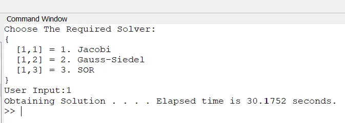

2. Transient-State

Main Script (it also contains the explicit scheme)

%Transient State Analysis
clear
close
clc

% Defining the domain and convergence criteria
L = 1; %m
nx = 31;
ny = nx;
x = linspace(0,L,nx);
y = linspace(0,L,ny);
h = x(2) - x(1);
alpha = 1.4;
tol = 1e-4;
count = 0;
t_start = 0;
t_end = 1;
err = 1;

% Initializing the temperature field with BCs
T = zeros(nx,ny);
T(1,2:end-1) = 900; %Bottom
T(end,2:end-1) = 600; %Top
T(2:end-1,1) = 400; %Left
T(2:end-1,end) = 800; %Right
T(1,1) = 650; T(1,end) = 850; T(end,end) = 700; T(end,1) = 500; %Corners
Tmid = []; %Centre node

% User input for the solver and scheme selection
list1 = {'Explicit scheme','Implicit scheme'};
list2 = {'Jacobi method','Gauss-Siedel method','SOR method'};
printf('Please Provide Input As Prompted\n')
disp(list1)
numerical_scheme = input('Choose a Numerical Scheme:');
if numerical_scheme == 2
  disp(list2)
  iterative_solver = input('Choose an Iterative Solver:');
else
  continue;
endif
disp('Obtaining a Solution . . . . ')
w=1.26;
% Computing through different solvers
if numerical_scheme==1
    % Explicit scheme
    dt = h^2/(4*alpha);
    t = t_start:dt:t_end;
    nt = length(t);
    K1 = alpha*dt/(h^2); tic;
    % Time loop
    for k=1:nt
        % Store the temperature values from previous time-step
        Told = T;
        % Space loop
        for i=2:nx-1
            for j=2:ny-1
                dT = Told(i-1,j) + Told(i+1,j) + Told(i,j-1) + Told(i,j+1);
                T(i,j) = (1-4*K1)*Told(i,j) + K1*dT;
            end
        end
        Tmid = [Tmid, T(x==0.5,y==0.5)];
        count = count + 1;
    end
    comp_time = toc;
elseif numerical_scheme==2
    % Implicit scheme
    dt = 0.01;
    t = t_start:dt:t_end;
    nt = length(t);
    K1 = alpha*dt/(h^2); tic;
    % Time loop
    for k=1:nt
        T_prev_dt = T; err = 1;
        % Convergence loop
        while err>=tol
            if iterative_solver==1
                [T, err] = jacobi_implicit(T,T_prev_dt,nx,ny,K1);
            elseif iterative_solver==2
                [T, err] = gauss_siedel_implicit(T,T_prev_dt,nx,ny,K1);
            elseif iterative_solver==3
                [T, err] = SOR_implicit(T,T_prev_dt,nx,ny,K1,w);
            end
            count = count+1;
        end
        Tmid = [Tmid, T(x==0.5,y==0.5)];
    end
    comp_time = toc;
end

figure(1)
contourf(x,y,T,'ShowText','on');
c = colorbar;
colormap(jet);
set(get(c,'label'),'string','Contour: Temperature (K)','FontSize',14);
xlabel('X (m)','FontSize',14); ylabel('Y (m)','FontSize',14);
if numerical_scheme==1
    str = {['Temperature contour at t = ',num2str(t_end),' using explicit scheme takes ',num2str(comp_time),'s']};
    text = ['Transient_analysis_',list1{numerical_scheme},'.png'];
elseif numerical_scheme==2
    str = {['Temperature contour at t = ',num2str(t_end),' using implicit scheme and ',list2{iterative_solver},' takes ', num2str(comp_time),'s']};
    text = ['Transient_analysis_',list1{numerical_scheme},'_',list2{iterative_solver},'.png'];
end
title(str,'FontSize',11)
saveas(1,text)

Function for transient Jacobi Iterator

%Jacobi Iterator for Implicit Method
function [T, err] = jacobi_implicit(T,T_prev_dt,nx,ny,K1)
    % Store the temperature values from previous iteration
    Told = T;
    % Space loop
    for i=2:nx-1
        for j=2:ny-1
            dT = Told(i-1,j) + Told(i+1,j) + Told(i,j-1) + Told(i,j+1);
            T(i,j) = (1/(1+4*K1))*T_prev_dt(i,j) + (K1/(1+4*K1))*dT;
        end
    end
    % Compute the error
    err = max(abs(T(i,j)-Told(i,j)));
end

Function for transient Gauss-Siedel Iterator

%Gauss-Siedel Iterator for Implicit Method
function [T, err] = gauss_siedel_implicit(T,T_prev_dt,nx,ny,K1)
    % Store the temperature values from previous iteration
    Told = T;
    % Space loop
    for i=2:nx-1
        for j=2:ny-1
            dT = T(i-1,j) + Told(i+1,j) + T(i,j-1) + Told(i,j+1);
            T(i,j) = (1/(1+4*K1))*T_prev_dt(i,j) + (K1/(1+4*K1))*dT;
        end
    end
    % Compute the error
    err = max(abs(T(i,j)-Told(i,j)));
end

Function for transient SOR Iterator

%SOR method for Implicit Scheme
function [T, err] = SOR_implicit(T,T_prev_dt,nx,ny,K1,w)
    % Store the temperature values from previous iteration
    Told = T;
    % Space loop
    for i=2:nx-1
        for j=2:ny-1
            dT = T(i-1,j) + Told(i+1,j) + T(i,j-1) + Told(i,j+1);
            T(i,j) = (1-w)*Told(i,j) + w*((1/(1+4*K1))*T_prev_dt(i,j) +...
                        (K1/(1+4*K1))*dT);
        end
    end
    % Compute the error
    err = max(abs(T(i,j)-Told(i,j)));
end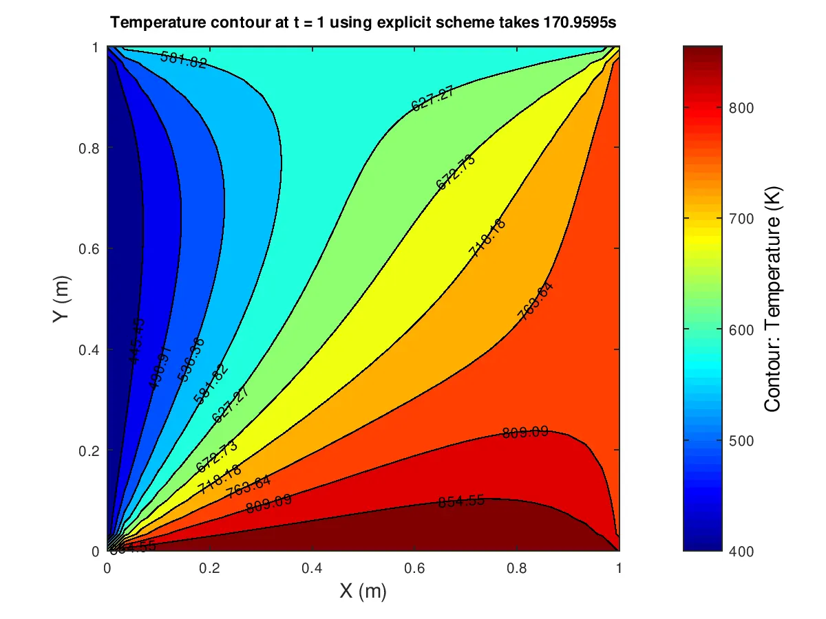

Results:

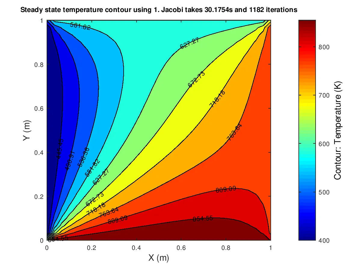
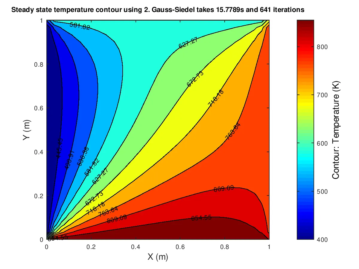
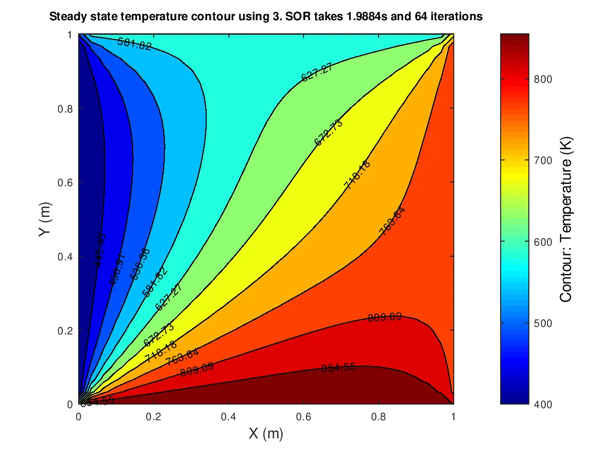
1. Steady-State

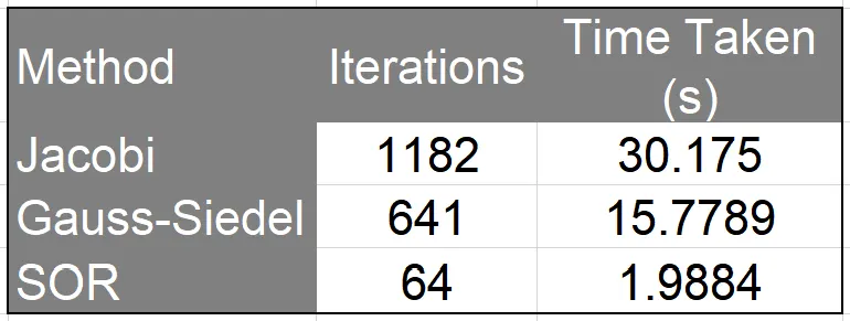
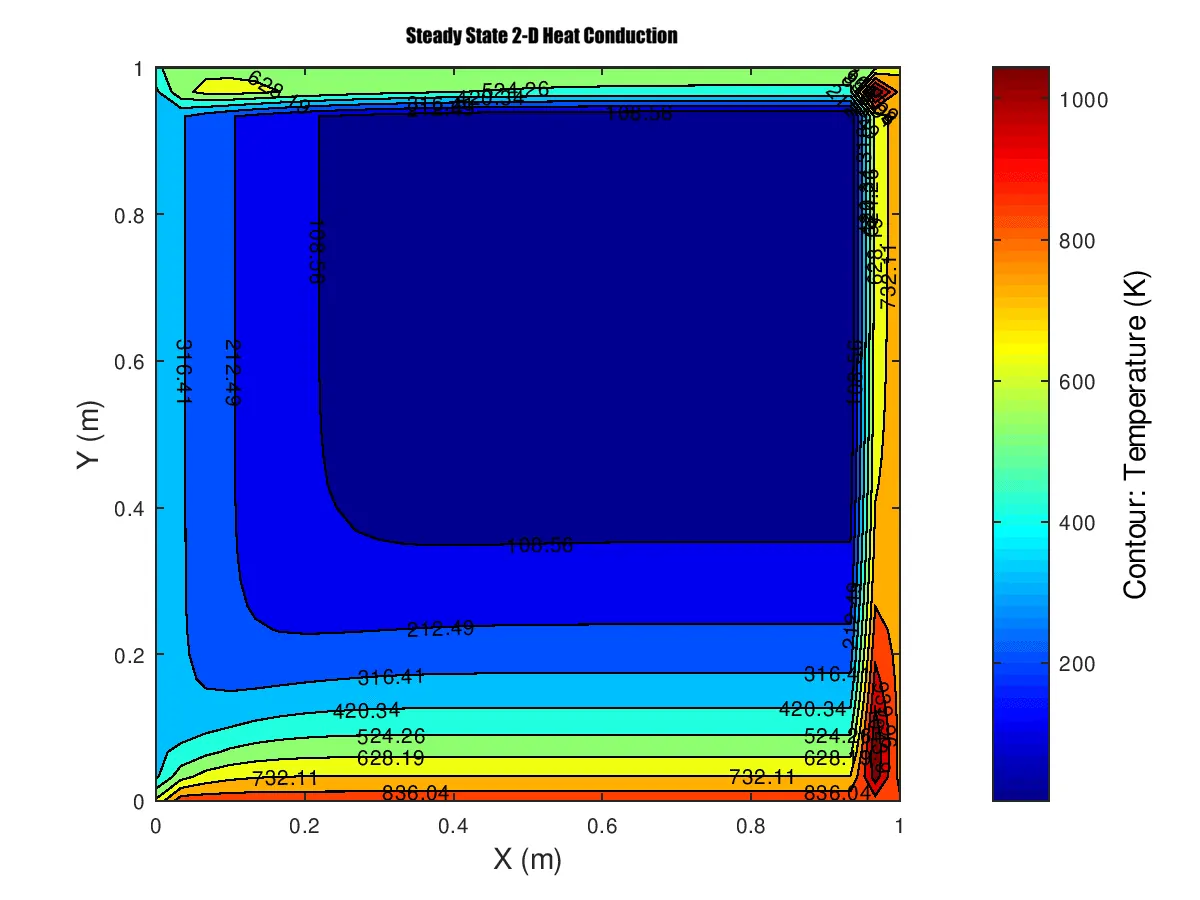
It is quite evident that Jacobi solver is the slowest one as it updates values from the previous iterations. Gauss-Siedal updates values in real time, hence, the number of iterations and time taken is reduced to half. The SOR method, which is improved Gauss-Siedal method, due to inclusion of a relaation factor was able to reduce the iterations drastically.

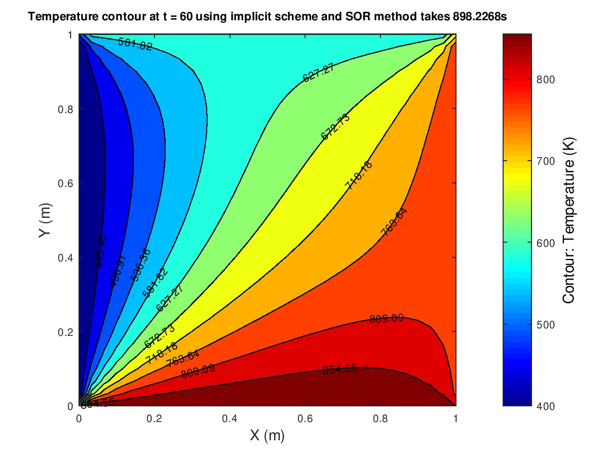
2. Transient-State

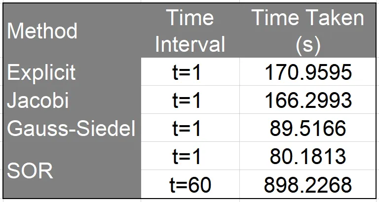
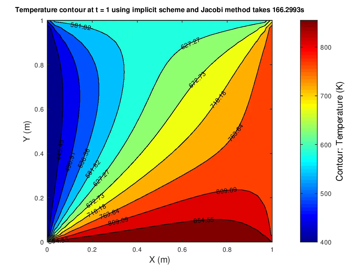
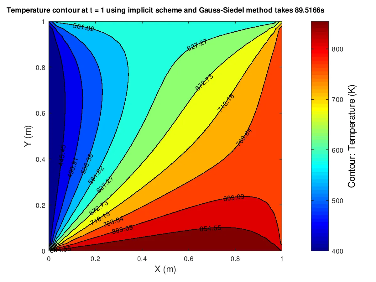
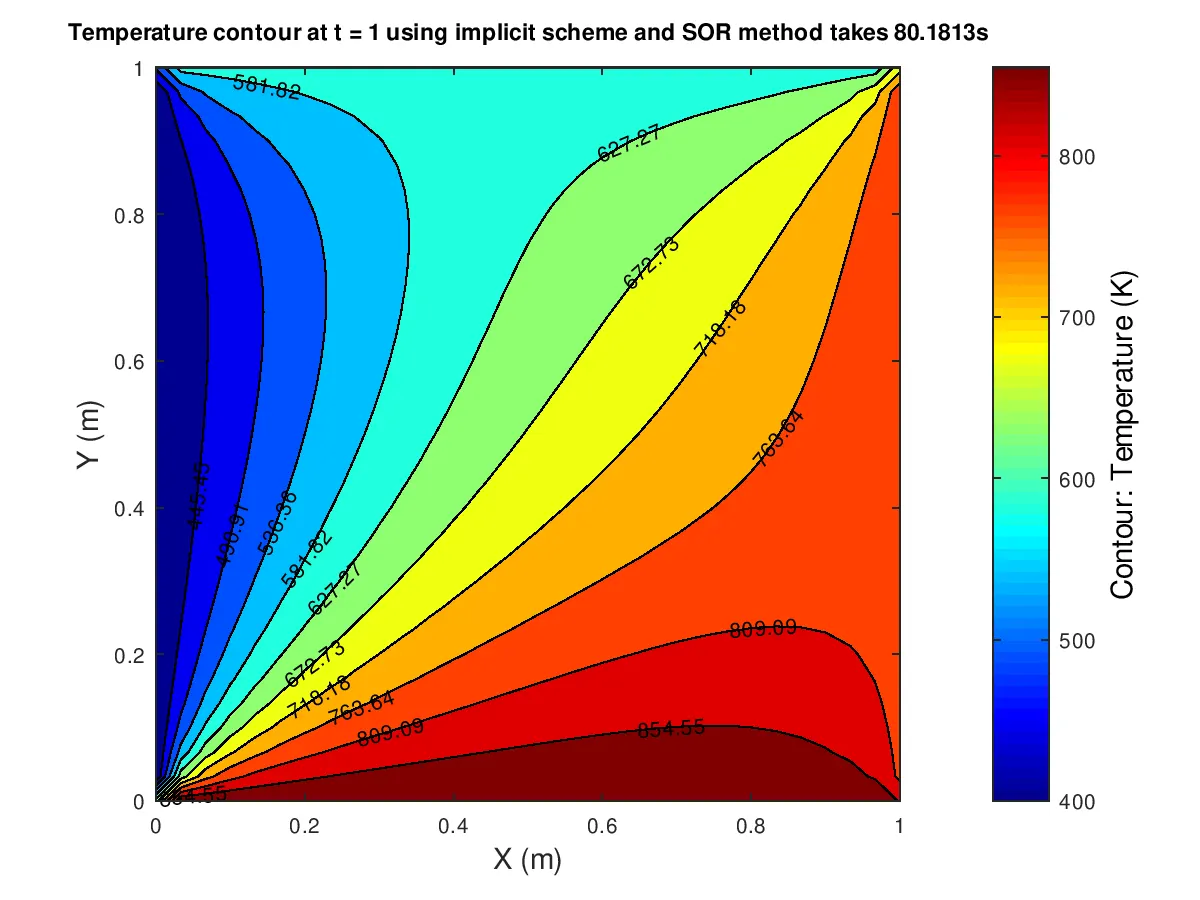
The same trends can be observed in transient conditions too. The explicit method too was quite fast. But this was so as this was a simple 2-D problem, in case of a complex problem or may be a 3-D problem, employing explicit method can be quite expensive than implicit scheme.

References:

• Introduction to CFD using MATLAB and OpenFOAM - Course provided by Skill Lync.
• GNU Octave
• Supporting Material: Fundamentals of Heat and Mass Transfer (SIE) - Yunus Cengel, Afshin Ghajar
• Supporting Material: Higher Engineering Mathematics - BS Grewal
• Supporting Material: Energy Engineering by VP Katekar Sir