Challenge

Week 5 - Genetic Algorithm

GGaneshram Devakumar12 Aug 2024

Objective of the Project - Writing a MATLAB code to optimize the Stalagmite function using Genetic algorithm and find the function’s global maxima. And also to plot the graph of F maximum v/s iterations for 3 different case studies.

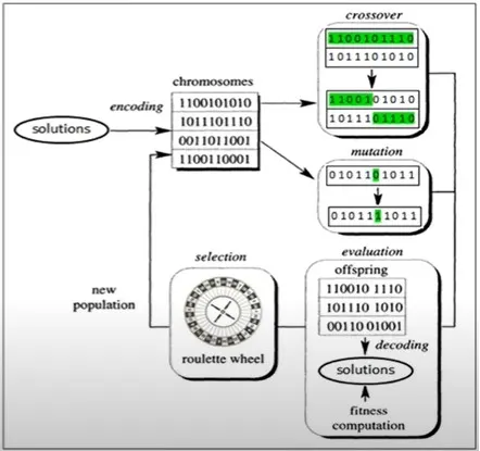
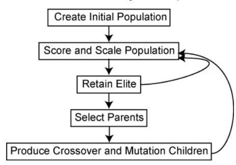
Genetic Algorithm Introduction - A genetic algorithm is a search heuristic that is inspired by Charles Darwin’s theory of natural evolution. This algorithm reflects the process of natural selection where the fittest individuals are selected for reproduction in order to produce offspring of the next generation.

Initial Population -

The population of individuals are maintained within search space. Each individual represents a solution in search space for given problem. Each individual is coded as a finite length vector (analogous to chromosome) of components. These variable components are analogous to Genes. Thus a chromosome (individual) is composed of several genes (variable components).

Fitness Function

The fitness function determines how fit an individual is (the ability of an individual to compete with other individuals). It gives a fitness score to each individual. The probability that an individual will be selected for reproduction is based on its fitness score.

Operators of Genetic Algorithms

Once the initial generation is created, the algorithm evolves the generation using following operators –

1) Selection Operator: The idea of selection phase is to select the fittest individuals and let them pass their genes to the next generation.

Two pairs of individuals (parents) are selected based on their fitness scores. Individuals with high fitness have more chance to be selected for reproduction.

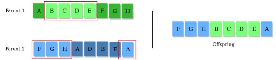
2) Crossover Operator: This represents mating between individuals. Two individuals are selected using selection operator and crossover sites are chosen randomly. Then the genes at these crossover sites are exchanged thus creating a completely new individual (offspring). For example –

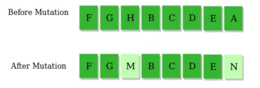
3) Mutation Operator: The key idea is to insert random genes in offspring to maintain the diversity in the population to avoid premature convergence. For example –

Genetic Algorithm (ga)Syntax -

x = ga(fun,nvars)-finds a local unconstrained minimum, x, to the objective function, fun. nvars is the dimension (number of design variables) of fun, where, fun- objective function and nvars-number of variables.

x = ga(fun,nvars,A,b,Aeq,beq,lb,ub)- defines a set of lower and upper bounds on the design variables, x, so that a solution is found in the range lb ≤ x ≤ ub. When there is no linear inequalities we set Aeq and Beq as null vector.

x = ga(fun,nvars,A,b,[],[],lb,ub,nonlcon,IntCon) or x = ga(fun,nvars,A,b,Aeq,beq,lb,ub,nonlcon,intcon,options) requires that the variables listed in IntCon take integer values.

Where, A and b are A=[] and b=[] if no linear inequalities.lb and ub are lower bound and upper bound. Lower bounds, and upper bound specified as a real vector or array of doubles.

The set of equation used in stalagmite function is shown in below image.

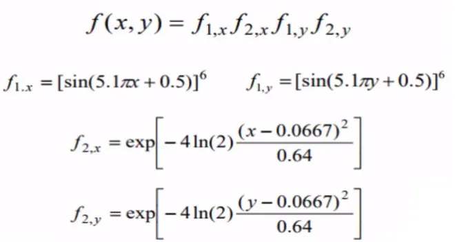
Stalagmite Function -

function [f] = stalagmite(input_vector)

f1x = (sin((5.1*pi).*input_vector(1)+0.5)).^6;

f1y = (sin((5.1*pi).*input_vector(2)+0.5)).^6;

f2x = exp((((input_vector(1)-0.0667).^2)/0.64).*(-4*log(2)));

f2y = exp((((input_vector(2)-0.0667).^2)/0.64).*(-4*log(2)));

f1=f1x*f1y*f2x*f2y;

f=-f1;

end

MATLAB code for Global Optimization -

%% Global Optimization using genetic algorithm

clear all

close all

clc

% Defining our search space

x = linspace(0,0.6,150); % X variables from 0 to 0.6 between 150 values

y = linspace(0,0.6,150); % y variables from 0 to 0.6 between 150 values

num_cases = 60 % To run the Genetic algoritam for 60 times

% creating a 2D mesh

[xx, yy] = meshgrid(x,y); % Transforming x,y 1D array into 2D array

% Evaluating the stalagmite function

for i = 1 : length(xx) % Assigning the value of xx in each iteration till length of xx

for j = 1 : length(yy) % Assigning the value of yy in each iteration till length of yy

input_vector(1) = xx(i,j);

input_vector(2) = yy(i,j);

f(i,j) = stalagmite(input_vector); % Assigning value of xx,yy into finction stalagmite for each iteration

end

Study #1 - Without Boundary Conditions

%% Study of Genetic algoritam without boundary conditions

tic

for i = 1 : num_cases;

[input, fopt(i)] = ga(@stalagmite,2); % fopt = optimum value of stalgmite function

xopt(i) = input(1);

yopt(i) = input(2);

end

figure(1)

subplot(2,1,1) % creating multiple polts in a same figure window by adjusting row

hold on

surfc(xx,yy,f) % Surface plotting the XX,YY and f (calculated using the stalagmite function)

xlabel('x value');

ylabel('y value');

title ('Genetic algoritam without boundary conditions')

shading interp % eliminate the grids in stalagmites and giving smooth plots

plot3(xopt,yopt,fopt,'marker','x','markersize',5,'markerfacecolor','m')

subplot(2,1,2) % creating multiple polts in a same figure window by adjusting row

hold on

% To plot for F maximun v/s No. of iterations

plot(fopt)

xlabel('No. of iterations');

ylabel('Function maximum');

study_time1 = toc

Study #2- With Upper and Lower Boundary Conditions

%% Study of Genetic algoritam with upper and lower bounds

tic

for i = 1 : num_cases

[input, fopt(i)] = ga(@stalagmite,2,[],[],[],[],[0;0],[0.6;0.6]);

xopt(i) = input(1);

yopt(i) = input(2);

end

figure(2)

subplot(2,1,1) % creating multiple polts in a same figure window by adjusting row

hold on

surfc(xx,yy,f) % Surface plotting the XX,YY and f (calculated using the stalagmite function)

xlabel('x value');

ylabel('y value');

title ('Genetic algoritam with bounded Inputs')

shading interp % eliminate the grids in stalagmites and giving smooth plots

plot3(xopt,yopt,fopt,'marker','x','markersize',5,'markerfacecolor','m')

subplot(2,1,2) % creating multiple polts in a same figure window by adjusting row

hold on

% To plot for F maximun v/s No. of iterations

plot(fopt)

xlabel('No. of iterations');

ylabel('Function maximum');

study_time2 = toc

Study #3- With Increased population

%% Study of Genetic algoritam with increasing iterations

options = optimoptions('ga')

options = optimoptions(options,'PopulationSize',120)

tic

for i = 1 : num_cases

[input, fopt(i)] = ga(@stalagmite,2,[],[],[],[],[0;0],[0.6;0.6],[],[],options);

xopt(i) = input(1);

yopt(i) = input(2);

end

figure(3)

subplot(2,1,1) % creating multiple polts in a same figure window by adjusting row

hold on

surfc(xx,yy,f) % Surface plotting the XX,YY and f (calculated using the stalagmite function)

xlabel('x value');

ylabel('y value');

title ('Genetic algoritam with increased populations')

shading interp % eliminate the grids in stalagmites and giving smooth plots

plot3(xopt,yopt,fopt,'marker','x','markersize',5,'markerfacecolor','m')

subplot(2,1,2) % creating multiple polts in a same figure window by adjusting row

hold on

% To plot for F maximun v/s No. of iterations

plot(fopt)

xlabel('No. of iterations');

ylabel('Function maximum');

study_time3 = toc

Study #4- With Increased population from 120 to 240

%% Study of Genetic algoritam with increasing population from 120 to 240

options = optimoptions('ga')

options = optimoptions(options,'PopulationSize',240)

tic

for i = 1 : num_cases

[input, fopt(i)] = ga(@stalagmite,2,[],[],[],[],[0;0],[0.6;0.6],[],[],options);

xopt(i) = input(1);

yopt(i) = input(2);

end

figure(4)

subplot(2,1,1) % creating multiple polts in a same figure window by adjusting row

hold on

surfc(xx,yy,f) % Surface plotting the XX,YY and f (calculated using the stalagmite function)

xlabel('x value');

ylabel('y value');

title ('Genetic algoritam with increased populations')

shading interp % eliminate the grids in stalagmites and giving smooth plots

plot3(xopt,yopt,fopt,'marker','x','markersize',5,'markerfacecolor','m')

subplot(2,1,2) % creating multiple polts in a same figure window by adjusting row

hold on

% To plot for F maximun v/s No. of iterations

plot(fopt)

xlabel('No. of iterations');

ylabel('Function maximum');

study_time4 = toc

Stepwise explanation of the program

For Global optimization using genetic algorithm, search space created using the linspace command, and meshgrid command is used to transform 1D in to 2D array
A sub program is created to evaluate stalagmite function and result is stored in f variable. those variables are plotted to show the 3d representation of stalagmite function.

Output 1 -

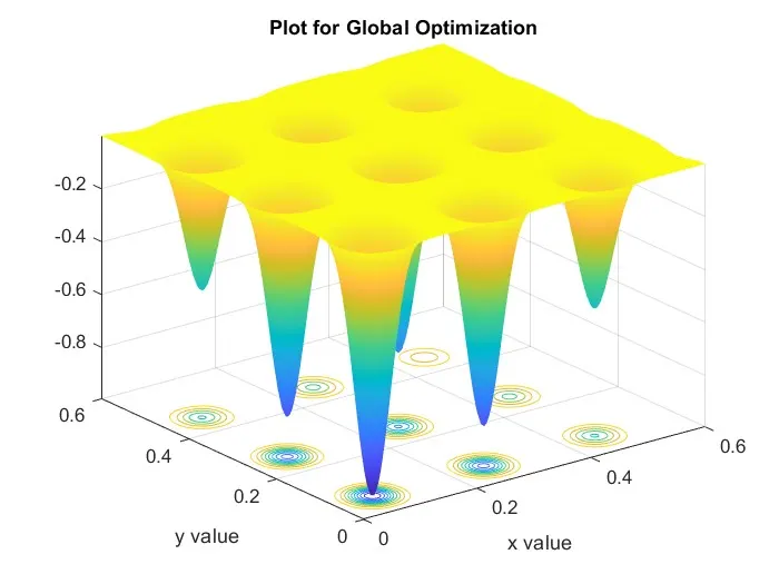
Study 1 – Statistical behaviour (Without Boundary Conditions)

In study #1 'ga' solver is iterated for 60 times, and in this case no limits are provided.
'ga' solver returns two outputs, one is the function value and other is the coordinates. Value of function is stored in 'fopt(i)' and coordinates are stored in 'xopt' and 'yopt' respectively. This loop is run for 60 times and results are plotted.
Figure 1 holds two plots and equally dived using subplot command. one showing the 3d representation of stalagmite with optimization results and other showing the function value
'Plot3' command is used to plot a set of coordinates connected by line segments and Time taken for 60 iteration is measured using tic' and 'toc' command
Results were found outside our search space (0 to 0.6) due to no upper and lower limit provided

Output 2 -

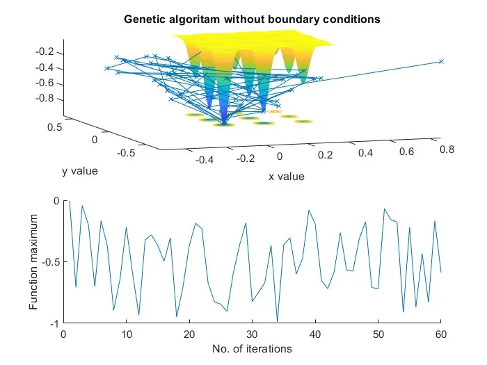
Study 2 – Upper and Lower Boundary Conditions

In study #2 'ga' solver is run with upper and lower limits which will narrow the search space
Four null vectors are passed in the solver syntax because there is no linear inequality involved in the stalagmite function.

Again, the loop is run for 60 times and 'Plot3' command is used to plot a set of coordinates connected by line segments and Time taken for 60 iteration is measured using tic' and 'toc' command

Output 3 -

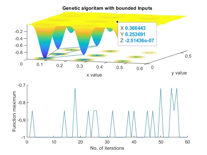
Study 3 – With Increased population

In study #3 the 'ga' solver is run with the bounded inputs along with the increased population size -120
Population Size specifies how many individuals are there in each generation. With a large population size, the genetic algorithm searches the solution space more thoroughly, thereby reducing the chance that the algorithm returns a local minimum that is not a global minimum. However, a large population size also causes the algorithm to run more slowly.
Optimoptions command is used to create optimization options.
'Plot3' command is used to plot a set of coordinates connected by line segments and Time taken for 60 iteration with increased population size is measured using tic' and 'toc' command

Output 4 -

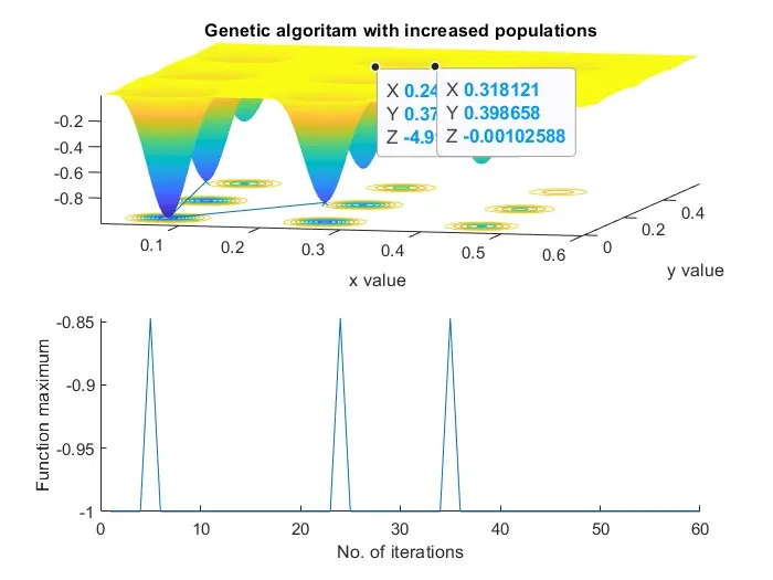
Output 5 - Population size further increased to 240

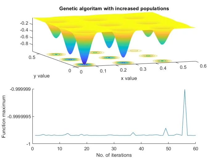
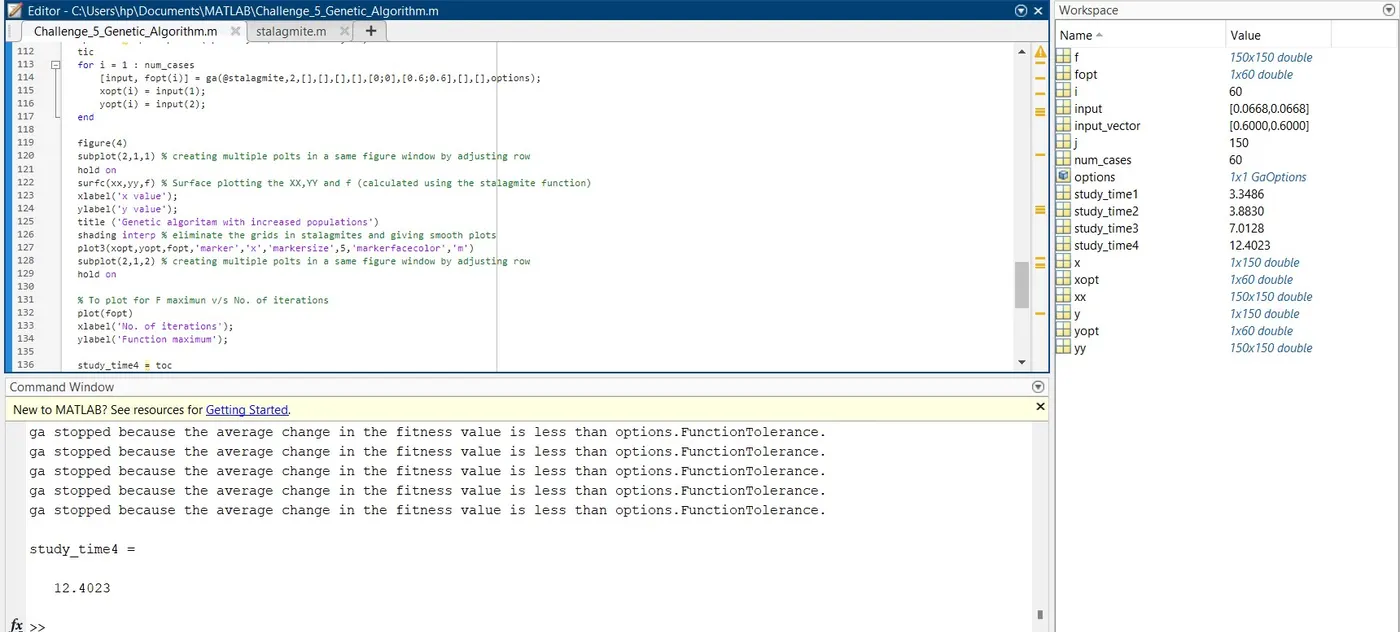
Output -6 - Final results with study time of all cases

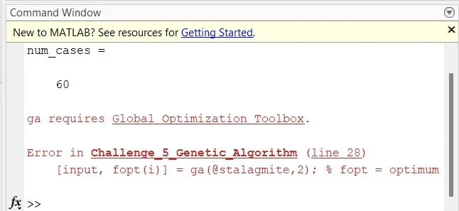
Error - Facing following error while solving ga, After add-on the 'Global Optimization Toolbox" I can able to solve the Ga

References -

1.https://in.mathworks.com/help/gads/what-is-the-genetic-algorithm.html

2.https://in.mathworks.com/help/gads/how-the-genetic-algorithm-works.html#f6243

3.https://www.youtube.com/watch?v=MLPHLm56inQ&t=3s

4.https://towardsdatascience.com/introduction-to-genetic-algorithms-including-example-code-e396e98d8bf3

5.https://www.geeksforgeeks.org/genetic-algorithms/

6.https://in.mathworks.com/help/gads/ga.html#mw_4a8bfdb9-7c4c-4302-8f47-d260b7a43e26

Week 5 - Genetic Algorithm

Ship work like this
in your own course.

Talk to a career counsellor

Ship work like thisin your own course.

Talk to a career counsellor

Ship work like this
in your own course.