Challenge

Project 1 - Data Handling and Interpolation

GGaneshram Devakumar5 Sept 2024

MATLAB

Objective of the Project

Solving the simple harmonic oscillator equation using ‘ode45’ and ‘ode23’
Program to determine the evaluated data using ‘polyfit’ and ‘polyval’
Evaluating the function and finding the local minima and global maxima
Brief note on ‘Contour’ command and illustrating with example

Objective 1 - Solving the simple harmonic oscillator equation using ‘ode45’ and ‘ode23’

Function - 'ode_func'

function [dx_dt] = ode_func(t,x,m,k)

x1 = x(1)

dx1_dt = x(2)

dx2_dt =((-k * x(1)) /m)

[dx_dt] = [dx1_dt;dx2_dt];

end

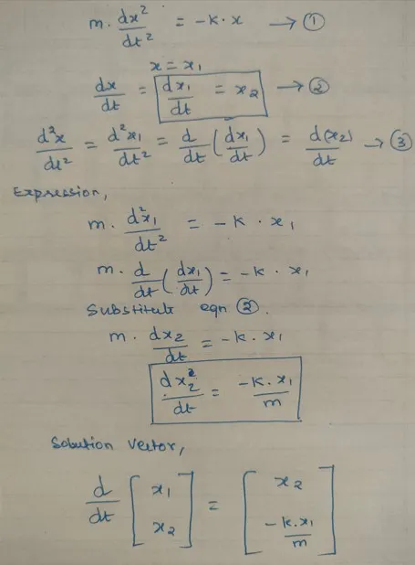
Function definition -

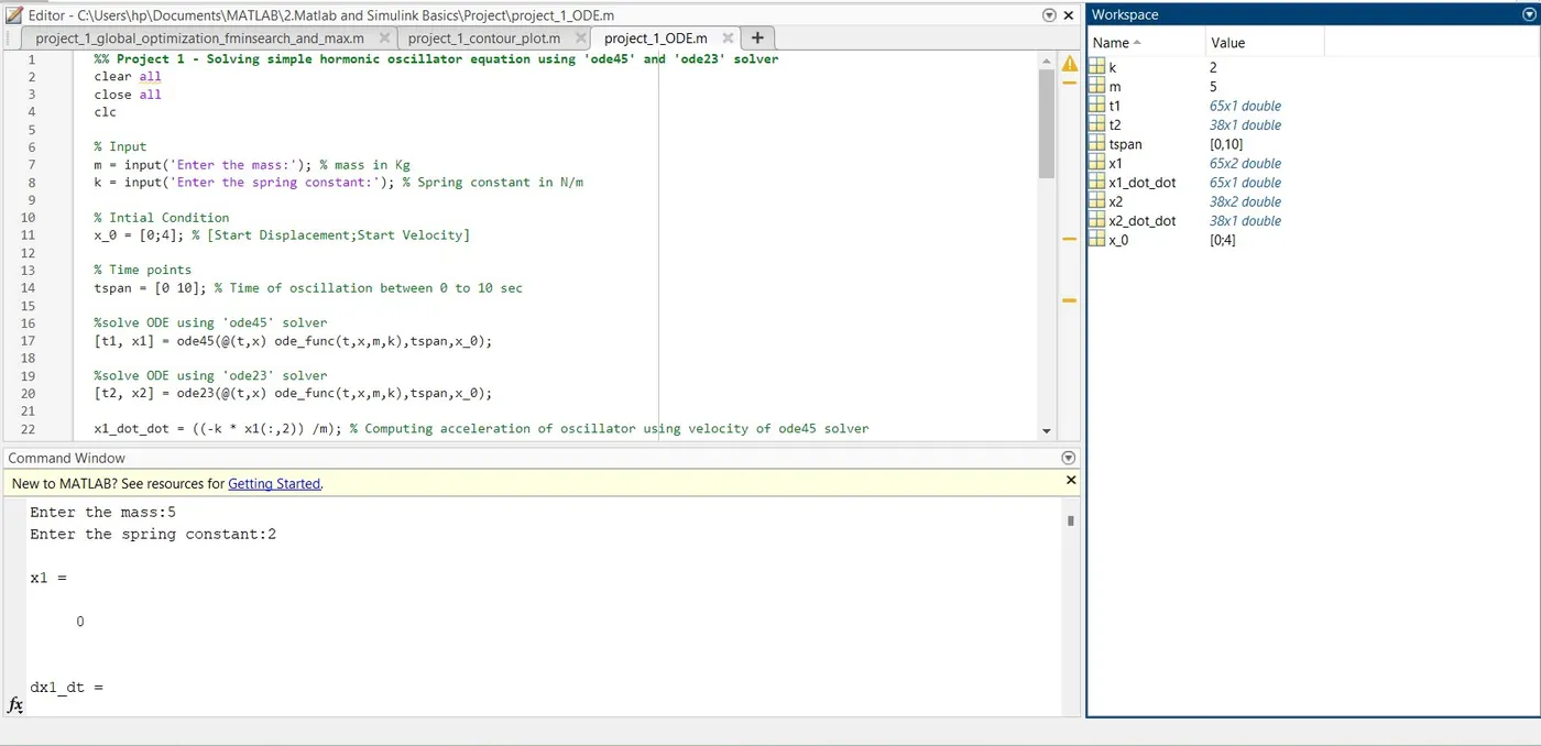
MATLAB Code –

%% Project 1 - Solving simple hormonic oscillator equation using 'ode45' and 'ode23' solver

clear all

close all

clc

% Input

m = input('Enter the mass:'); % mass in Kg

k = input('Enter the spring constant:'); % Spring constant in N/m

% Intial Condition

x_0 = [0;4]; % [Start Displacement;Start Velocity]

% Time points

tspan = [0 10]; % Time of oscillation between 0 to 10 sec

%solve ODE using 'ode45' solver

[t1, x1] = ode45(@(t,x) ode_func(t,x,m,k),tspan,x_0);

%solve ODE using 'ode23' solver

[t2, x2] = ode23(@(t,x) ode_func(t,x,m,k),tspan,x_0);

x1_dot_dot = ((-k * x1(:,2)) /m); % Computing acceleration of oscillator using velocity of ode45 solver

x2_dot_dot = ((-k * x2(:,2)) /m); % Computing acceleration of oscillator using velocity of ode23 solver

% Plotting the x,x_dot,x_dot_dot for ode45

figure(1)

plot(t1,x1(:,1),'b--','LineWidth',2); % plot between time and postion results of ode45 solver

hold on

plot(t1,x1(:,2),'m:','LineWidth',2); % plot between time and velocity results of ode45 solver

plot(t1,x1_dot_dot,'y-','LineWidth',2); % plot between time and acceleration

xlabel('Time in sec','FontSize',12,'Color','r');

ylabel('Value of x','FontSize',12,'Color','r');

title(['Solving simple Hormonic Oscillator using ode45']);

legend('x', 'x-dot','x-dot-dot');

hold off

% Plotting the x,x_dot,x_dot_dot for ode23

figure(2)

plot(t2,x2(:,1),'b--','LineWidth',2) % plot between time and postion results of ode23 solver

hold on

plot(t2,x2(:,2),'m:','LineWidth',2) % plot between time and velocity results of ode23 solver

plot(t2,x2_dot_dot,'y-','LineWidth',2) % plot between time and acceleration

xlabel('Time in sec','FontSize',12,'Color','r')

ylabel('Value of x','FontSize',12,'Color','r')

title(['Solving simple Hormonic Oscillator using ode23'])

legend('x', 'x-dot','x-dot-dot')

hold off

Code Explanation –

Defining the user input by using 'input' command
Defining the initial condition as [0,4]( i.e. [Start Displacement ; Start Velocity]) and time span from 0 to 10 sec.
Definition the function ‘ode_func.m’ to solve the expression
Using ‘ode45’ command given expression is solved for user input initial condition and time span.
Using ‘ode23’ command given expression is solved for user input initial condition and time span.
Using the results ‘x_dot_dot’ computed
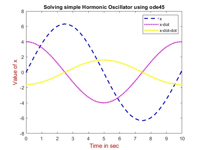
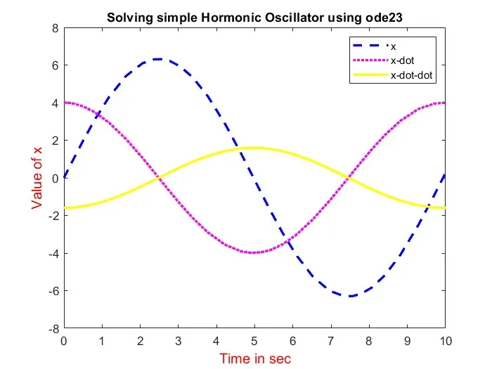
The results of two solvers plotted separately (position, velocity and acceleration of simple hormonic oscillator) with proper annotation, label, title and legend

Comparing 'ode45' and 'ode23'plot –

ode23 is a three-stage, third-order, Runge-Kutta method. ode45 is a six-stage, fifth-order, Runge-Kutta method.
ode45 does more work per step than ode23, but can take much larger steps.
For differential equations with smooth solutions, ode45 is often more accurate than ode23. In fact, it may be so accurate that the interpolant is required to provide the desired resolution.
ode45 is the anchor of the differential equation suite. The MATLAB documentation recommends ode45 as the first choice. And Simulink blocks set ode45 as the default solver.

Output -

Objective 2 - Program to determine the evaluated data using ‘polyfit’ and ‘polyval’

MATLAB Code –

% Program to determine the evaluated data using ‘polyfit’ and ‘polyval’

clear all

close all

clc

% Opening the excel file and save the data in 'data' variable

data = xlsread("ISA_PROJECT1_Q2_DATA.xlsx");

Alt = data(:,1); % 1st column of 'data' variable is Altitude data

Temp = data(:,2); % 2nd column of 'data' variable is Temperature data

% Finding the polynomial coeffficient using the data

p = polyfit(Alt,Temp,3); % considered as a 3rd order polynomial hence n =3

% Finding the validated values of Temp.

Temp_eval_data = polyval(p,Alt); % using the coefficients and Alt data finding evalyuated Temperature data

% Finding the goodness of fit using system identification inbuit command

disp('Goodness of fit')

GOT = goodnessOfFit(Temp,Temp_eval_data,'MSE') % comparing the original data with evaluated data

% Plotting the evauated results and actual resutls

plot(Alt,Temp,'m--',LineWidth=2); % plotting the actual/loaded data

grid;

hold on

plot(Alt,Temp_eval_data,'k:',LineWidth=2); % plotting the evaluated data

xlabel('Altitude in m','FontSize',12,'Color','b');

ylabel('Temperature in K','FontSize',12,'Color','b');

legend('Original Data','Evaluted Data');

title('Polynomial function');

hold off

% Saving the interpolation in 'text' file

fid = fopen('polyval_evaluated_results.txt','w')

fprintf(fid,'%s\n','Polynomial evaluated data using polyval')

fprintf(fid,'%16s %16s\n','Alt','Temp_eval_data')

% for loop to write the data line by line for each iteration

for i = 1 : length(Alt) % Iteration length as Alt data length

fprintf(fid,'%16.5f %16.5f\n',Alt(i),Temp_eval_data(i)); % space after %f will create space after wirting each numbers in text file

end

fclose (fid); % closing the opened file

Code Explanation –

Opening the excel file using 'xlsread' command.
Assign the variable data to 'Alt' and 'Temp' with respective column.
Using the 'polyfit' command finding the polynomial coefficients with degree of polynomial fit as 3.
Using the 'polyval' command with 'Altitude' data and polynomial coefficients, evaluated temperature values are captured.
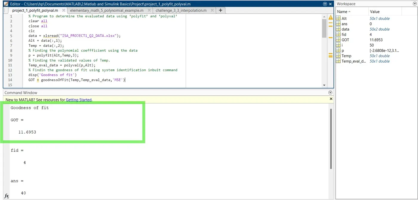
Finding the goodness of fit using system identification command 'goodnessOfFit'. it will measure the quantitative representation of the closeness of actual data to evaluated data. If fit '0', represents the maximum closeness of actual data and evaluated data.
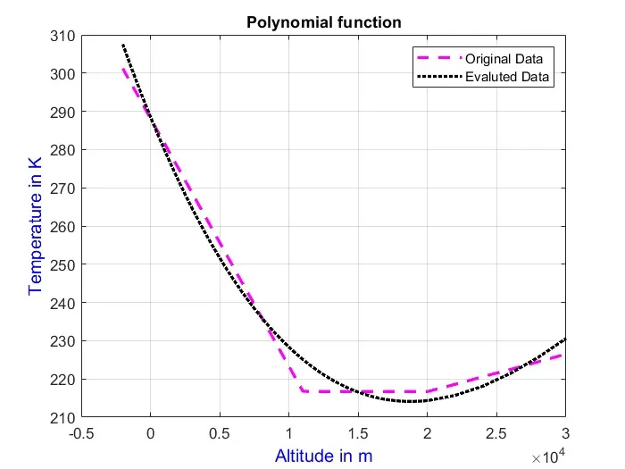
Plotting results of actual data and evaluated data to compare with proper annotation, title, label and legend.
Opening the file in new text format ‘polyval_evaluated_results.txt’ using ‘fopen’ command with proper header.
Annotating the header for each column values.
Saving the each values of data one by one using for loop with iteration as length of Alt. with proper alignment of data in text file.
Closing the opened text file using ‘fclose’ command.

Output -

Output save file - ' polyval_evaluated_results.txt'

Polynomial evaluated data using polyval

Alt Temp_eval_data

-2000.00000 307.53623

-1500.00000 302.54252

-1000.00000 297.71072

-500.00000 293.03882

0.00000 288.52480

500.00000 284.16666

1000.00000 279.96239

1500.00000 275.90997

2000.00000 272.00740

2500.00000 268.25266

3000.00000 264.64375

3500.00000 261.17865

4000.00000 257.85535

4500.00000 254.67185

5000.00000 251.62613

5500.00000 248.71617

6000.00000 245.93998

6500.00000 243.29554

7000.00000 240.78084

7500.00000 238.39386

8000.00000 236.13261

8500.00000 233.99506

9000.00000 231.97921

9500.00000 230.08304

10000.00000 228.30455

10500.00000 226.64172

11000.00000 225.09255

11500.00000 223.65503

12000.00000 222.32713

12500.00000 221.10686

13000.00000 219.99220

13500.00000 218.98114

14000.00000 218.07167

14500.00000 217.26179

15000.00000 216.54947

15500.00000 215.93271

16000.00000 215.40950

16500.00000 214.97783

17000.00000 214.63568

17500.00000 214.38105

18000.00000 214.21193

18500.00000 214.12630

19000.00000 214.12216

19500.00000 214.19749

20000.00000 214.35029

22000.00000 215.69589

24000.00000 218.12006

26000.00000 221.49413

28000.00000 225.68941

30000.00000 230.57722

Objective 3 - Evaluating the function and finding the local minima and global maxima

MATLAB Code –

% Global optimization to find the Global Maxima and Local Minima

clear all

close all

clc

% defining the expression y = sin(x²)+cos(x)-2*sin(x)*cos(x)

fun = @(x) sin(x.^2) + cos(x) - 2*sin(x).*cos(x);

% input the value of x

x = [0:pi/100:2*pi];

% Computing the expression as a function of x

y = fun(x)

% plotting the x & y results

plot(x,y);

grid;

hold on

xlabel('x');

ylabel('y');

title('Global Optimization ');

% Finidng the Global maxima using 'max' command

[ymax,imax] = max(y);

xmax = x(imax); % from the postion of x, finding the value of x

% Finidng the Local minima using 'fminsearch' command

[xmin, ymin] = fminsearch(fun, 5); % from the plot location of local minimum at approximate position is 5

[x1min, y1min] = fminsearch(fun, 3); % from the plot location of local minimum at approximate position is 3

[x2min, y2min] = fminsearch(fun, 2); % from the plot location of local minimum at approximate position is 2

% Getting the x anf y value of global maxima point to mention the text in plot

text(xmax,ymax,'Global Maxima','HorizontalAlignment','center');

% Getting the x anf y value of local minima point to mention the text in plot

text(xmin,ymin,'Local Minima','HorizontalAlignment','center');

% Getting the x anf y value of local minima point to mention the text in plot

text(x1min,y1min,'Local Minima','HorizontalAlignment','center');

% Getting the x anf y value of local minima point to mention the text in plot

text(x2min,y2min,'Local Minima','HorizontalAlignment','center');

hold off

Code Explanation –

Defining the given function 'y= sin(x²) +cos(x) - 2 sin(x) cos(x)' as a function
Input the x values for 0 to 2Pi range in a interval of pi/100
Computing the y values using the 'fun' expression as a function of 'x'
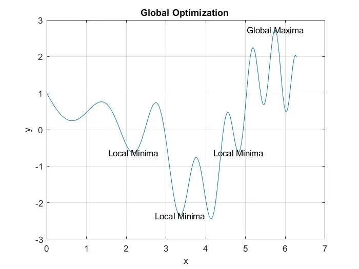
Plotting the results of x and y with proper annotation, label and title
Using 'Max' command, finding the global maxima at respective index position of x and value of y and using x index position values of x stored in 'xmax'
Using 'fminsearch' command, all local minima's captured with the guess values from the plot
With x,y coordinates of of 'global maxima' and 'local minima' points, text is created in the plot

Output -

Reference - https://in.mathworks.com/help/optim/ug/local-vs-global-optima.html

Objective 4 - Brief note on ‘Contour’ command and illustrating with example

Brief Note on 'Contour' -

A contour plot is a graphical technique for representing a 3-dimensional surface by plotting constant z slices, called contours, on a 2-dimensional format. The contour plot is an alternative to a 3-D surface plot.

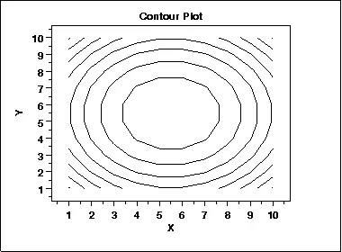
The graph shows values of the Z variable for combinations of the X and Y variables. The X and Y values are displayed along the X and Y-axes, while contour lines and bands represent the Z value. The contour lines connect combinations of the X and Y variables that produce equal values of Z.

Contour plots are particularly helpful when you need to identify combinations of X and Y that produce beneficial or required values of Z. This contour plot shows that the surface is symmetric and peaks in the centre.

The contour lines and bands make it easy to find combinations that yield the values you need.

Use a contour plot to assess the following features of your dataset:

Explore the relationship between three variables on a single chart.

View combinations of X and Y that produce desirable outcome values.

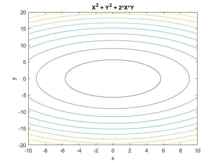
Example MATLAB Code –

% Contour plot

clear all

close all

clc

% input

x = [-10:0.1:10];

y = [-20:0.2:20];

% Transforming 1-dimension array omto 2-dimensional array using meshgrid

[X Y] = meshgrid(x,y);

% Evaluating the Z variable as a function of X & Y

Z = X.^2 + Y.^2 + 2*X*Y;

% creating contour plot

contour(X,Y,Z)

xlabel('x')

ylabel('y')

title('X^2 + Y^2 + 2*X*Y')

Output -

Project 1 - Data Handling and Interpolation

Ship work like this
in your own course.

Talk to a career counsellor

Ship work like thisin your own course.

Talk to a career counsellor

Ship work like this
in your own course.