Week 5 - Genetic Algorithm
AIM - Genetic Algorithm
Objective -
- Write a code in MATLAB to optimise the stalagmite function and find the global maxima of the function.
- Clearly expalin the concept of genetic algorithm in your own words and also explain the syntax for ga in MATLAB in your report.
- Make sure that your code gives the same output, even if it is made to run several times.
- Plot graphs for all 3 studies and for F maximum vs no. of iterations. Title and axes labels are a must, legends could be shown if necessary.
Theory -
Optimization - Optimization is the process of selection from the set of values for the imposed targets and the constraints.
Processes handling many parameters , where its integrated with each other and affects one another in all aspects.
It's been very difficult to manage and select the appropriate range of values for the defined targets and constraints.
• To make this process ease , optimization techniques helps us to find a way to get the best out of it .
Population algorithms : An algorithm that maintains an entire set of candidate solutions , and each solution corresponds to a unique point in the search space of the problem known as population based algorithm.
Some of the notable population based algorithms are as follows ,
1. Genetic Algorithm
2. Differential Evolution
3. Particle Swarm Optimization
Applications of optimization
• Mechanics
● Economics and finance
• Machine Learning
● Artificial Intelligence
• Controls Engineering
The flowchart explains the working of genetic algorithm.
The three main processes going behind the GA solvers such as ;
1. Selection
2. Crossover
3. Mutation
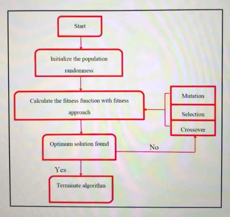
Outline of the algorithm
- creating a random initial population .
- creates a sequence of new populations .
- Scores each member of the current population by computing its fitness value.
- Selects members , called parents , based on their best fitness value .
Creating next generation
Selection : It defined the selection of parents for the next generation using selection function / fitness function which will be based on the fitness value.
Cross over : Crossover enables the algorithm to extract the best characters from different individuals and recombine them into potentially superior children.
Mutation : Mutation adds to the diversity of a population and thereby increases the likelihood that the algorithm will generate individuals with better fitness values.
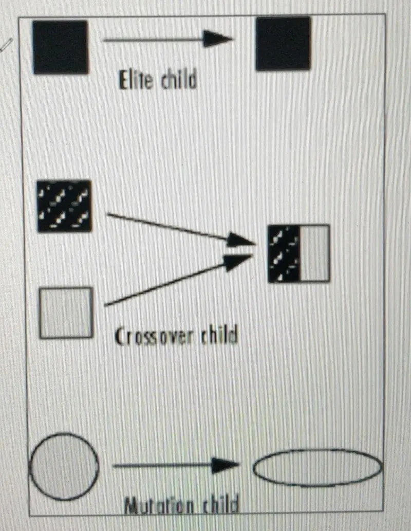
- Types of children produced for next generation from the current population parents as follows ,
- Elite child : Individuals having best fitness values
- Crossover child : Created by combining the parents
- Mutation child : Created by doing random changes to the single parent
- GA Syntax
| x = ga ( fun , nvars , A , b , Aeq , beq , lb , ub , nonlcon , options ) |
fun = Objective function
nvar = Number of Variables ( specified as positive integer )
A,b = Linear inequality constraints ( A = Real matrix ; b = Real vector )
Aeq , beq = Linear equality constraints ( A = Real matrix ; b = Real vector )
Lb , ub = Lower bounds and upper bounds
nonlcon = Nonlinear constraints
options = Optimization options
PROCEDURE -
- While start any program its better to close all window and erase previous calculations, so we use these three commands-
- clear - this command clear all previous data stored in the workspace window.
- close - this command close all the previous figure and plot.
- clc - this command clear all data in command window.
Defining the input space Give the possible range of inputs for the ga solver as like shown .
|
clear
close
clc
% difining input spaces
x = linspace(0,0.6,150);
y = linspace(0,0.6,150);
num_cases = 50;
|
● This input will be considered as the space for the algorithm to solve .
● It should be the practical range suitable for the problem .
|
f1x = ( sin ( ( 5.1 * pi * x ) +0.5 ) ) ^ 6 ;
f1y = ( sin ( ( 5.1 * pi * y ) +0.5 ) ) ^ 6 ;
f2x = exp ( -4 * log ( 2 ) * ( ( ( x - 0.0667 ) ^ 2 ) /0.64 ) ) ;
f2y = exp ( -4 * log ( 2 ) * ( ( ( y - 0.0667 ) ^ 2 ) /0.64 ) ) ;
f = - ( flx * fly * f2x * f2y ) ;
|
Evaluating the objective function
Using a for loop will be helpful to cover the two dimensional input ( both x and y ) .
For every point in the xy plane stalagmite function will be called to calculate the ' f ' value .
[ xx , yy ] = meshgrid ( x , y ) ;
|
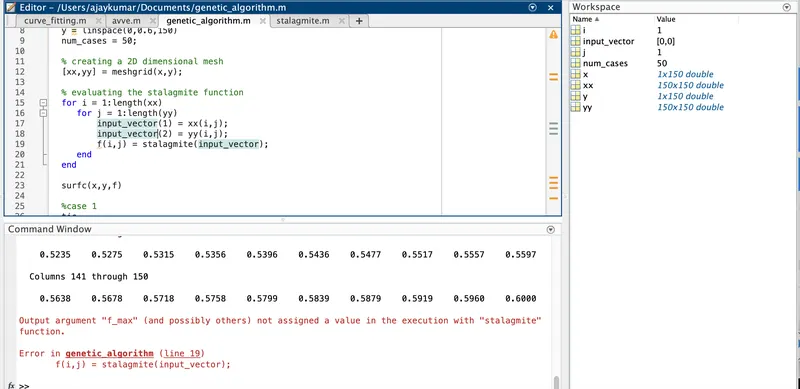
% evaluating the stalagmite function
for i = 1:length(x)
for j = 1:length(y)
input_vector(1) = xx(i,j);
input_vector(2) = yy(i,j);
f(i,j) = stalagmite(input_vector);
end
end
|
CASE 1 :-
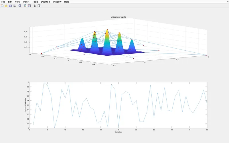
Unbounded GA study
|
% (case 1) for Performing unbounded GA
for k = 1 :num_cases
[inputs,fopt(k)] = ga(@stalagmite,2)
xopt(k)= inputs(1);
yopt(k) = inputs(2);
end
tic
|
|
figure(1)
subplot(2,1,1)
% f = -f for rotating plots
surfc(x,y,-f)
hold on
shading interp
plot3(xopt,yopt,-fopt,'marker','o','markersize',5,'MarkerFaceColor','r')
title('unbounded inputs')
subplot(2,1,2)
plot(-fopt)
xlabel('iteration')
ylabel('function maximum')
|
- subplot( m , n , p ) - Divides the current figure into an m -by- n grid and creates axes in the position specified by p .
The first subplot is the first column of the first row, the second subplot is the second column of the first row, and so on.
- Surfc - MATLAB graphics defines a surface by the z-coordinates of points above a rectangular grid in the x-y plane.
f = -f , here we convert the function in negative for rotaing the plot.
- hold on - here hold on stand for retains plots in the current axes so that new plots added to the axes do not delete existing plots.
- plot3( X , Y , Z )- plots coordinates in 3-D space and marker stand for Adding markers to a line plot can be a useful way to distinguish multiple lines or to highlight particular data points.
- markersize - is used to control the overall size of markers, just like the overall width of a line with LineWidth or font size.
- markerfacecolor - You can use the "MarkerFaceColor" and "Color" properties of the plotted line or lines in order to fill in the markers with the same color as the default marker edge color.
And than we plot the function in a axis or y axis
- xlabel('iteration') - hare we plot the Iteration is a key element in much of technical computation.
Examples involving the Golden Ratio introduce the Matlab assignment statement, for and while loops, and the plot function.
- ylabel('function maximum') - now we plot the functions maximum value in y axis or find the function maximum value.
CASE 2 :-
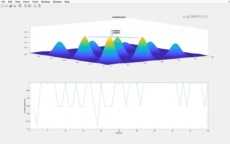
BOUNDED GA STUDY
BOUNDED CASE : ● Here in the GA syntax the lower and upper bounds are defined.
● With defined bounds of x from ' 0 to 0.6 ' and bounds of y from 0 to 0.6' results in the better optimization.
|
% (case 2) for Performing bounded GA
for i = 1:num_cases
[inputs,fopt(i)] = ga(@stalagmite,2,[],[],[],[],[0;0],[0.6;0.6]);
xopt(i) = inputs(1);
yopt(i) = inputs(2);
end
|
When the bounds are not confined the results of GA tends to be random
- The outputs tends to be unstable .
- The upper and lower bounds been defined and so the solver tends to converge and will be close to accuracy .
- The bounds should be added within the x and y range.
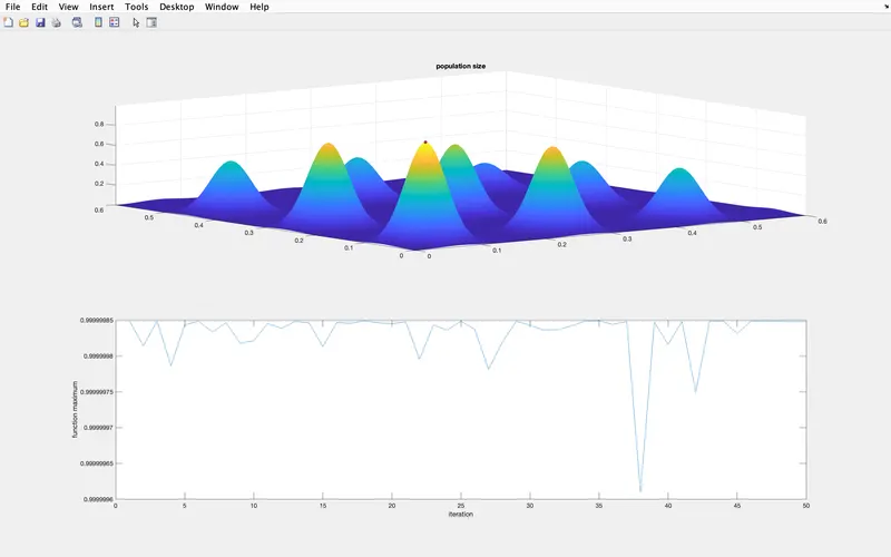
- The default population size for ga solver is 50 . Population size can be added as the feature using options in the ga syntax .
- Increase the population size until the single optimum point is achieved .
- Increasing population size will increase the simulation time .
|
tic
for i = 1:num_cases
[optimoptions,fopt(i)] = ga(@stalagmite,2,[],[],[],[],[0;0],[0.6;0.6],[],[],options);
xopt(i) = inputs(1);
yopt(i) = inputs(2);
end
case3_time = toc
|