Week 3 - Solving second order ODEs

AIM - Solving second order ODEs

OBJECTIVE - to write a program that solves the following ODE. This ODE represents the equation of motion of a simple pendulum with damping.

THEORY - Differential equation is the one involved with one or more derivatives including the study of changes.

• A derivative or a slop is ratio of change in 'y' to change in 'x' respectively.
• Differentiating the function y=f(x), leads to the ''first order derivative'' dy/dx.

There are two types differential equations

• Ordinary differential equations(ODE)

A differential equation containing one or more functions of one independent variables.

• Partial differential equations(PDE)

A differential equation containing one or more functions of two or more independent variables.

Solving ordinary differential equation (ODE).

• Numerical techniques to solve ODES

• Solving differential equations analytically would be a tedious process .
• There are certain numerical methods to solve the differential equations computationally
• The Differential equations should be discretised and will be represented as linear algebraic forms known as 'Numerical Discretisation '

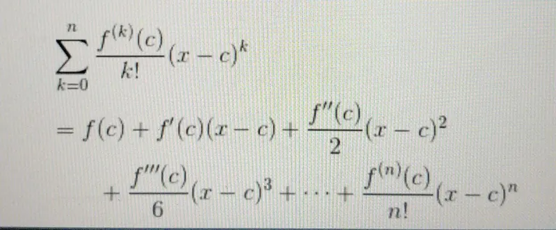
• Taylor series approximation " is the significant way to get the numerical solutions to the differential equations

• The Taylor series of a function is an infinite sum of terms that are expressed in terms of the function's derivatives at a single point.
• It will be used in numerical approximations of any function .

• Runge kutta method ( RK )

• RK method is one of the most familiar methods of approximation which is an extended " Euler method " , derived from the " Taylor series " .
• It overcomes the demerits of ' Taylor series approximation ' by excluding the calculations of ' higher order derivatives ' , in turn it can be used for any functions having high accuracies .

• First Order RK / Euler method Euler - Method in nothing but the first order RK method involving only the first order derivative.

• It is formed from the taylor series as follows ,

Yeuler = Yk + ∆xƒ( xk , Yk )

• 4th Order RK method - ODE45 uses an RK4 ( 4 step Euler ) method to perform numerical integration at each point to find the solution .

ay/dx=f(x,y)

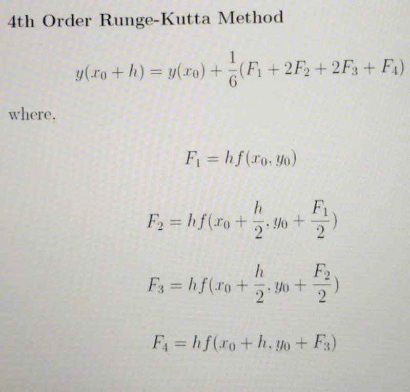
Working of ODE45 ODE45 -Working of ODE45 ODE45 is used to solve higher order non - stiff ODES.

• Non - stiff - solutions vary rapidly through out.
• Stiff - solutions vary rapidly along with smooth portions and hence smaller steps needed to capture the behaviour.

PROCEDURE -

• While start any program its better to close all window and erase previous calculations, so we use these three commands-

1. clear - this command clear all previous data stored in the workspace window.

2. close - this command close all the previous figure and plot.

3. clc - this command clear all data in command window.

Now iscretisation of an ODE.

The differential equation is as follows

the equation can not directly solved in matlab so we should convert the equation in 1st order differential equation by using the concept of state space as shown

• Displacement = theta =theta1
• velocity = d(theta)/dt = theta2 -----------(1)

d^2(theta)/dt^2 = (-b/ml)(theta2)-(g/l)sin(theta1)------------(2)

• Now define inputs or state definations which includes as follows,

1. Damping Coefficient b = 0.5 Nm/s

2. Acc due to gravity g = 9.81 m/s^2

3. Length of the string = 1 m

4. Mass of bob m = 1 kg

5. Initial displacement = 0 rad

6 . Initial Velocity = 3 rad / s

7. Time , tspan = 0 to second

• Now solving ODE45 -

-The above code shows the definition of the ODE45 Solver in matlab.

-The ODE45 integrate the function using numerical integration technique Runge Kutta Method.

• Here in solving ode we use function as shown below

Now plotting - Ploting for figure 1

Now using 'for loop' - For loop runs a piece of code for predetermined numbers of times.

For making an ANIMATION -

Following terminology are used for creating Animation.

M(ct)=getframe(gcf);

• getframe - It capture the figure as frame.
• gcf - It refers to the current figure handle in MATLAB where it captures and in turn give the current figure to capture it as a frame for movie creation.
• Counter variable(ct) - It helps in proper indexing in which the capture frame will be indexed sequentially.

Plotting - Now plotting of pendulum

Now creating move creation.

• movie(M) = plays the movie frames in array 'M' once.
• VideoWriter= This command will creat a video file of specified name and format.
• open= Opens the specified file (video file).
• writeVideo= writes the created video file with the frames captured in a the 'M' array.
• close= Close the specified file.

And finally the video file will be saved in the program path.

CODE -

RESULTS -

usp=sharinghttps://drive.google.com/file/d/1Yqbr3HOzetKnziXvDfJpg-i5ZXkD49MD/view?usp=sharing