Project 1 - Parsing NASA thermodynamic data

AIM - Parsing NASA thermodynamic data

OBJECTIVE -

1. Write a function that extracts the 14 co-efficients and calculates the enthalpy, entropy and specific heats for all the species in the data file.

The formulae are shown below.

Here R is the universal gas constant, T is the temeprature

The FIRST 7 coefficients are HIGH-temperature coefficients and the SECOND 7 coefficients are LOW-temperature coefficients.

Also use the LOCAL TEMPERATURE RANGES which is unique for each individual species, not the GLOBAL TEMPERATURE RANGE.

2. Calculate the molecular weight of each species and display it in the command window.

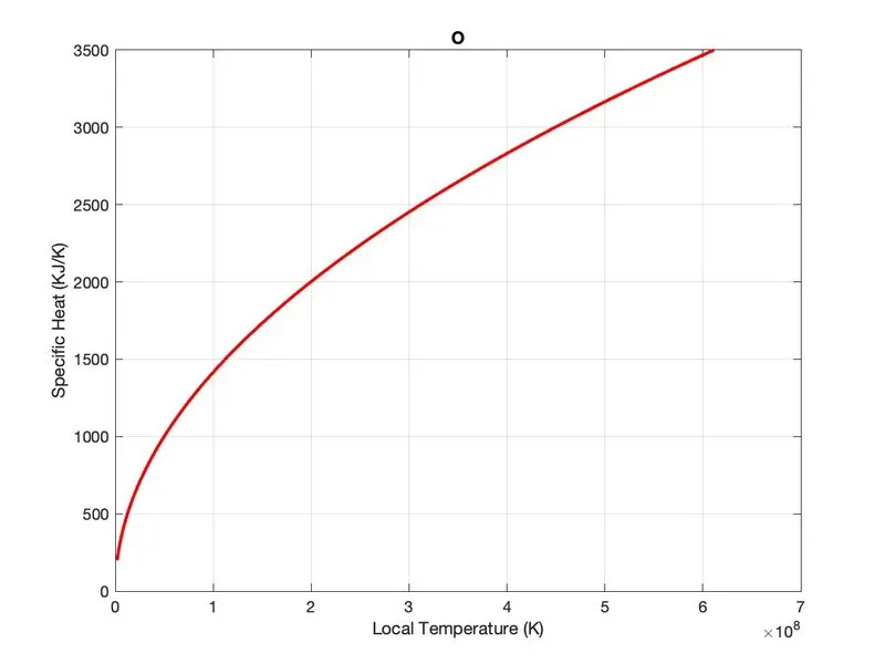
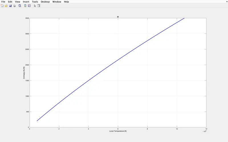
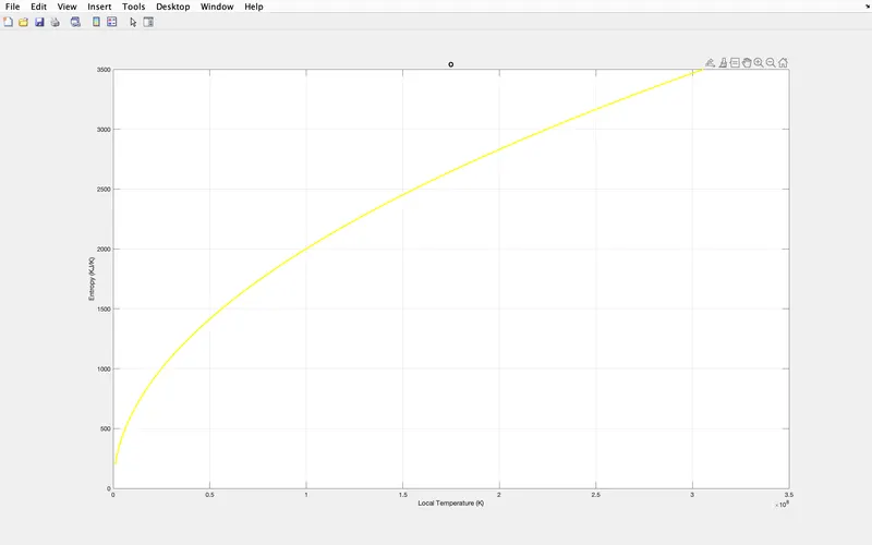
3. Plot the Cp, Enthalpy and Entropy for the local temperature range (low temperature : high temperature) specific for each species.

4. Save the plots as images with appropriate names and dump them in separate folders for each species with suitable name. All these should be generated automatically.

5. The main program that you will submit will just take the "THERMO.dat" file as an input and generate Cp, H and S plots.

6. Please write a detailed report to describe your logic.

THEORY -

file parsing - This deals with the field of computational linguistics where it commonly defines the natural language processing.

Natural language processing ( NLP ) , is concerned with programming the computers to process and analyse the human written language.

Parser helps to split the large input data into smaller data and will process the data.

Why file parsing ?

• Parsing is necessary because different application needs the data to be in different forms.
• Parsing allows transforming the data in a way that can be understood by a specific software.
• The obvious example is programs they are written by humans , but they must be executed by computers .
• Parsing helps to automate the certain ings , and also reduces the human effort. And can be used for the applications of machine learning , automation etc ;

PROCEDURE -

• While start any program its better to close all window and erase previous calculations, so we use these three commands-

1. clear - this command clear all previous data stored in the workspace window.
2. close - this command close all the previous figure and plot.
3. clc - this command clear all data in command window.

• The task includes the parsing of a ' NASA thermodynamic file ' , and to calculate the specific heat ( cp ) , Enthalpy ( H ) , Entropy ( S ) for defined local temperatures.
• The file includes the 53 different species having its own local temperature range.
• The file includes the NASA thermodynamic data.

1st we have to reading the file - The file should be loaded and opened in the script using the ' fopen ' command.
And the lines necessary for the calculation should be get from the file using ' fgetl '.

f = fopen ( ' THERMO.dat ' , ' r ' )

fgetl ( f )

• Now Using strsplit command beacause it is string type so, spliting by space because it common in this line

• The temperature values available in the header line of every species is known as local temperature.
• It includes ' low ' , ' high ' , ' middle ' temperatures as in the order.
• Will be used in the calculation of Cp , H , S.

• Now we can extract the coefficient values - The coefficients are of two categories , such as high temperature coefficients ( first 7 coefficients ) and low temperature coefficients ( second 7 coefficients ).

• Now Calculation of cp(specific heat), h(enthalpy), s(entropy)

• Now Temperature array creation

• Next step is plotting and saving the figures

By using mkdir command and cd commands

In the last END the for loop.

CODE -

% file parsing

clear

close

clc

% file read

f = fopen('THERMO.dat','r')

for i = 1:5

fgetl(f);

end

for i = 1:53

b = fgetl(f);

% Using strsplit command beacause it is string type so, spliting by space

% because it common in this line

a = strsplit(b,' ');

species_name = a{1};

% To Calculate the molecular weight of each species created and function to

% find all molecular weight

% % molecular_wt = calc_of_molecular_weight(species_name);

% Extraction of local temperature

low_temp = str2double(a{end-3});

high_temp = str2double(a{end-2});

mid_temp = str2double(a{end-1});

% now we can extract coefficient values

A = fgetl(f);

pos = strfind(A,'E');

% variable "a" represent the coefficent value

a1 = str2double(A(1:(pos(1)+3)));

a2 = str2double(A((pos(1)+4):(pos(2)+3)));

a3 = str2double(A((pos(2)+4):(pos(3)+3)));

a4 = str2double(A((pos(3)+4):(pos(4)+3)));

a5 = str2double(A((pos(4)+4):(pos(5)+3)));

B = fgetl(f);

pos2 = strfind(B,'E');

a6 = str2double(B(1:(pos2(1)+3)));

a7 = str2double(B(1:(pos2(1)+4):(pos(2)+3)));

a8 = str2double(B(1:(pos2(2)+4):(pos(3)+3)));

a9 = str2double(B(1:(pos2(3)+4):(pos(4)+3)));

a10 = str2double(B(1:(pos2(4)+4):(pos(5)+3)));

C = fgetl(f);

pos1 = strfind(C,'E');

a11 = str2double(C(1:(pos1(1)+3)));

a12 = str2double(C((pos1(1)+4):(pos1(2)+3)));

a13 = str2double(C((pos1(2)+4):(pos1(3)+3)));

a14 = str2double(C((pos1(3)+4):(pos1(4)+3)));

% R is universal gas number

% R = 8.314; % J/Mol*km(units)

% Calculation of cp(specific heat), h(enthalpy), s(entropy)

% Temperature array creation

T =linspace(low_temp,high_temp,500);

[cp,h,s] = calc_therm_properties(a1,a2,a3,a4,a5,a6,a7,a8,a9,a10,a11,a12,a13,a14,T,mid_temp);

mkdir(['/users/ajaykumar/Desktop/species/',species_name])

cd(['//Users/ajaykumar/Desktop/species/',species_name])

% Temperature v/s specific heat

figure(1)

plot(cp,T,'linewidth',2,'color','r')

title(species_name)

xlabel('Local Temperature (K)')

ylabel('Specific Heat (KJ/K)')

grid on

saveas(1,'specific heat','jpg')

% Temperature v/s Enthalpy

figure(2)

plot(h,T,'linewidth',2,'Color','b')

title(species_name)

xlabel('Local Temperature (K)')

ylabel('Enthalpy (KJ/K)')

grid on

saveas(1,'Enthalpy','jpg')

% Temperature v/s Entropy

figure(3)

plot(s,T,'linewidth',2,'Color','y')

title(species_name)

xlabel('Local Temperature (K)')

ylabel('Entropy (KJ/K)')

grid on

saveas(1,'Entropy','jpg')

end

RESULTS -

FIGURE(1)

FIGURE(2)

FIGURE(3)