Week 5 - Genetic Algorithm

Aim - To write a for stalagmite function and to calculate its global maxima value using MATLAB.

Theory -

• Genetic Algorithm (GA) is a search-based optimization technique based on the principles of Genetics and Natural Selection. It is frequently used to find optimal or near-optimal solutions to difficult problems which otherwise would take a lifetime to solve. It is frequently used to solve optimization problems, in research, and in machine learning.
• The genetic algorithm repeatedly modifies a population of individual solutions. At each step, the genetic algorithm selects individuals at random from the current population to be parents and uses them to produce the children for the next generation over successive generations, the population evolves toward an optimal solution.
• You can apply the genetic algorithm to solve a variety of optimization problems that are not well suited for standard optimization algorithms, including problems in which the objective function is discontinuous, non differentiable, stochastic, or highly non-linear. The genetic algorithm can address problems of mixed-integer programming, where some components are restricted to be integer-valued.
• The genetic algorithm uses the main types of rules at each step to create the ne generation from the current population

Selection rules: Select the individuals, called parents that contribute to the population at the next generation.

Crossover rules: Combine two parents to form children for the next generation

Mutation rules: Apply random changes to individual parents to form the children.

FITNESS FUNCTION:

The fitness function takes the solution as input and produces the suitability of the solution as the output. This evaluates how close the solution is to the optimal solution of the desired problem.

The syntax for GA in Matlab:

x=ga(fun,nvars,A,B,Aeq,Beq, lb, ub,nonicon,Intcon.options

• This syntax is explained as follows:
• ‘X’ is the variable to store the output of the genetic algorithm.
• ‘fun’ is the function handle to call the function.
• A and B are used to represent the linear inequalities of the function, if the linear inequalities do not exist, they can be set as empty[].
• Aeq and Beq are used to represent the equality constraints similarly, if the linear equalities do not exist, they can be set as empty[].
• ‘ib' and 'ub' are used to specify the upper and the lower bounds of the variables of the function.
• ‘nonlcon’ represents the non-linear constraints.
• ‘Intcon’ represents the integer constraint, such that the value of the function is an integer.
• ‘options’ used to provide the value of the default parameters used named parameters, if required to replace the default parameters. This is done by using the ‘optimoptions’.

SATALGMITE FUNCTION:

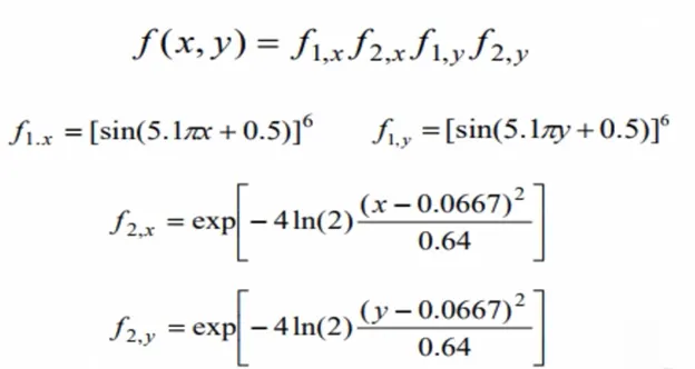
A stalagmite function generally refers to the function with which we are generating values over a stalagmite kind of surface for finding out the local and global maxima and minima of that particular given function.

Body content -

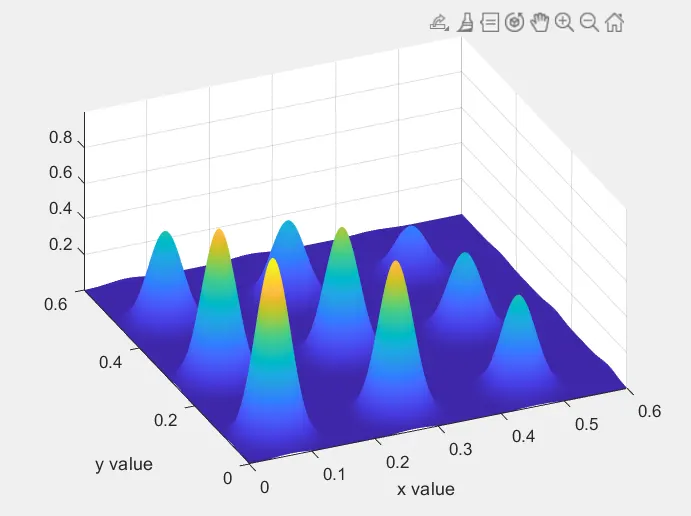
• For defining our search space,using the 'linspace command x and y variables are defined ranging from 0 to0.6 in 500 elements. Now using the "meshgrid" command a 2 dimensional mesh plane is generated for the code to run properly.
• Now for evaluating the stalagmite function two for loops are used, the values for two input variables are given by the 2 dimensiong mesh plane generated with the help of “meshgrid" command.

Code -

close all
clear all
clc

%defining our search space
x= linspace(0,0.6,500);
y= linspace(0,0.6,500);

%creating 2d mesh
[xx,yy]= meshgrid(x,y);

%Evaluating stalegmite function
for i = 1:length(yy);
for j = 1:length(xx);
input_vector(1)= xx(i,j);
input_vector(2)= yy(i,j);
f(i,j)= stalagmite1(input_vector);
end
end

surfc(xx,yy,f)
shading interp
[iput fval]= ga(@stalagmite1,2);
xlabel('x value');
ylabel('y value');

Result -

Case 1 -UNBOUNDED STATISTICAL BEHAVIOR:

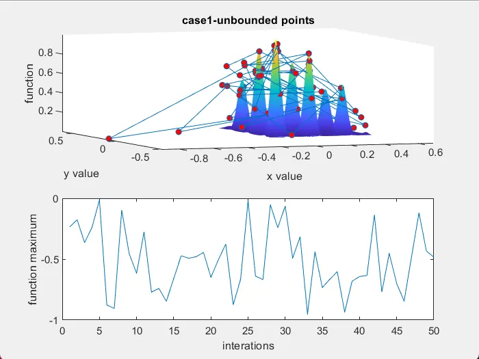
• Now starting with the first study that is unbounded statistical behavior. Here for defining the number of iterations a variable "num_cases" is used and is set to 50. For determining the time taken by then code to evaluate "tic" and "toc" command is used.
• The format of "ga" (genetic algorithm) used in this case is “[inputs, fopt] =ga (fun,nvars)”. Here inputs represent the values of the parameters x and y for which the function has the least value (fopt)”fun” is the function to be optimized, here it is a Stalagmite function, "nvars” the number of input variables, in this case its two “ input_vector(1)" and "input vector(2)”.
• Now for plotting the graph figure command is used for a new figure window, "subplot" is used for dividing the window in parts, and here it divides the figure window in two parts in the first two graphs are plotted in a single graph using the "hold” on command “surfc” command is used which plots a surface graph and the other graph is 3 dimensional line plot for this the command used is "plot3" X and Y label is given along with the title in the second half a ID plot is generated of valuesstored in "fopt" using the plot command and then label the x-axis and y-axis.

Code -

%study1 - Satistical Behaviour
num_cases = 50 ;
tic

for i = 1:num_cases;
[inputs1,fopt1(i)] = ga(@stalagmite1,2);
xopt1(i) = inputs1(1);
yopt1(i) = inputs1(2);
end
study_time1 = toc

%plotting
figure(2)
subplot(2,1,1)
hold on
surfc(xx,yy,-f)
xlabel('x value')
ylabel('y value')
zlabel('function')
shading interp
plot3(xopt1,yopt1,-fopt1,'marker','o','markersize',5,'markerfacecolor','r')
title('case1-unbounded points')
subplot(2,1,2)
plot(fopt1)
xlabel('interations')
ylabel('function maximum')

Result -

Case 2 -WITH UPPER AND LOWER BOUNDS:

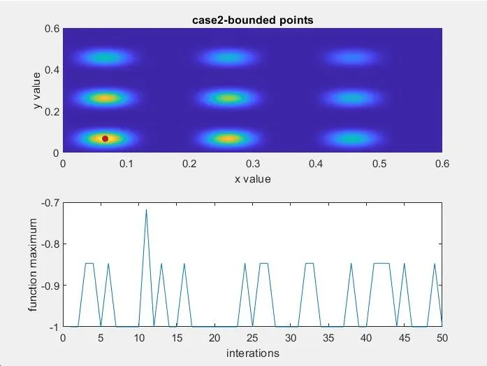
• Now for staring with the second study 'statistical behavior with upper and lower bound Here for defining the number of iterations a variable "num_cases is used and is set to 50. For determining the time taken by then code to evaluate "tic and toc" command is used
• The format of ga (genetic algorithm) used in this case is [inputs, fopt] = ga(fun,nvars A.b.Aeq.beq lb,ub) Here "inputs represents the values of the parameter and y for which the function has the least value (fopt) "fun" is the function to be optimized, here it is a Stalagmite function, "nvars in the number of input variables in this case its two, "input_vector(1)" and "input_vector(2) "A" is the linear inequality constraints real matrix, if there are none, then [],”b” is the linear inequality constraints real vector, if there are none, then []. "Aeq" is the linear inequality constraints real matrix, if there are none, then []; “beq" is the linear inequality constraints: real vector, if there are none, then [], "lb" is the lower bounds, specified as areal vector or array, "ub" is the upper bounds, specified as a real vector or array.
• Now for plotting the graphs, "figure command is used for a new figure window, “subplot" is used for dividing the window in parts, and here it divides the figure window In two parts. In the first half two graphs are plotted in a single graph using the "hold” on command, "surfc” command is used which plots a surface graph and the other graph is 3 dimensional line plat for this the command used is "plot3 X and Y label is given along with the title. Now in the second half a 1D plot is generated of values stored in “fopt” using the “plot” command and then label the x-axis and y-axis.

Code -

%Study2 - Satistical behaviour with upper and lower bounds
tic
for i = 1:num_cases;
[inputs2,fopt2(i)] = ga(@stalagmite1,2,[],[],[],[],[0;0],[0.6;0.6]);
xopt2 = inputs2(1);
yopt2 = inputs2(2);
end
study_time2 = toc

%plotting
figure(3)
subplot(2,1,1)
hold on
surfc(xx,yy,-f)
xlabel('x value')
ylabel('y value')
zlabel('function')
shading interp
plot3(xopt2,yopt2,-fopt2,'marker','o','markersize',5,'markerfacecolor','r')
title('case2-bounded points')
subplot(2,1,2)
plot(fopt2)
xlabel('interations')
ylabel('function maximum')

Result -

Case 3 - WITH INCREASED POPULATION:

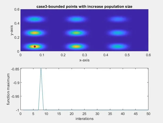
• Now for staring with the second study statistical behavior with increased population size. Here for defining the number of iterations a variable "num_cases” is used and is set to 50. For determining the time taken by then code to evaluate “tic and toc” command is used.
• The format of “ga “(genetic algorithm) used in this case is [inputs,fapt]=ga(fun,nvars,A,b,Aeq.beq.lb,ub.nonicon,intCon options)". Here inputs, fpt fun, nvars, A, b, Aeq, beq, lb and ub are same as mentioned as above,"nonicon” nonlinear constraints, specified as a function handle or function name, if there are none, then[], “intCon": integer variables, specified as a vector of positive integers, if there are none, then []. and "options" optimization options, specified as the out of optimizations or a structure.
• Now for plotting the graphs, "figure" command is used for a new figure window, subplot" is used for dividing the window in parts, and here it divides the figure window in two parts. In the first half two graphs are plotted a single graph using the "hold” on command, "surtc" command is used which plats a surface graph and the other graph is 3 dimensional line plot for this the command used is "plot3". X and Y label is given along with the title. Now in the second half 1D plot is generated of values stored in "fopt” using the "plot" command and then label the x-axis and y-axis.

Code -

%Study3 - Incresing GA interations
%in this, in addition to specify the bounds we also change the population

options = optimoptions('ga');
options = optimoptions(options,'populationsize',200);

tic
for i = 1:num_cases;
[inputs3,fopt3(i)] = ga(@stalagmite1,2,[],[],[],[],[0;0],[0.6;0.6],[],[],options);
xopt3 = inputs3(1);
yopt3 = inputs3(2);
end
study_time3 = toc

%plotting
figure(4)
subplot(2,1,1)
hold on
surfc(xx,yy,-f)
xlabel('x-axis')
ylabel('y-axis')
zlabel('function')
shading interp
plot3(xopt3,yopt3,-fopt3,'marker','o','markersize',5,'markerfacecolor','r')
title('case3-bounded points with increase population size')
subplot(2,1,2)
plot(fopt3)
xlabel('interations')
ylabel('function maximum')

Result -

Stalagmite function -

• Used to calculate f value for plotting graph.basically it will give z axis value.But the function gives minimum value and we want maximum value so modified function so it will give max value.

Code -

function[f]= stalagmite1(input_vector);
x=input_vector(1);
y=input_vector(2);

f1 = [sin(5.1*3.14*x + 0.5)]^6;
f2 = [sin(5.1*3.14*y + 0.5)]^6;
f3 = exp(-4*log(2)*((x-0.0667)^2/0.64));
f4 = exp(-4*log(2)*((y-0.0667)^2/0.64));
f5 = (f1*f2*f3*f4);
f=-f5;
end

Colculusion -

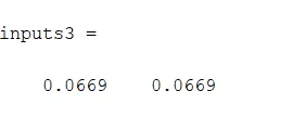
• We got the values at where function gives global maxima.