Week 3 - Solving second order ODEs

Aim - To solve ODE represents the equation of motion of a simple pendulum with damping.

Governing equation - Below equation of simple pendulum with damping.

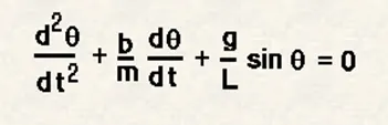
g = gravity in m/s2,

L = length of the pendulum in m,

m = mass of the ball in kg,

b=damping coefficient.

Objectives -

• To solve ODE represents the equation of motion of a simple pendulum with damping.
• Create animation of the motion of pendulum.

Body content -

• We have second order equation of motion of a simple pendulum.First we have to convert the second order euation into single order so it will become easy to solve equation.
• we have taken inputs like damping coefficent , angular velocity , angular displacement .
• we used ode45 which is inbuild ODE solver. It compares methods of orders four and five to estimate error and determine step size. ODE45 is so accurate that its default behavior is to use its interpolant to provide results at intermediate points.
• ODE45 stands for the Runge-Kutta(4,5) method. Such method is suited for solving ordinary differential equations by predictions.
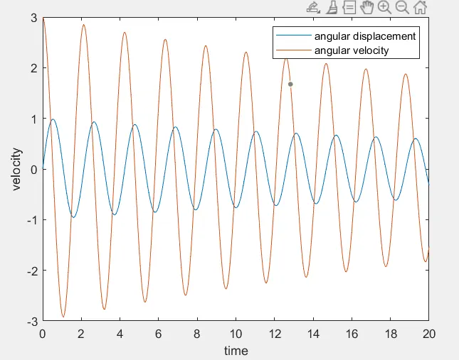
• With help of this solver we got angular velocity and displacement values with use of this we have plotted graph of them.
• For animation of pendulam motion we have fixed one end of pendulum and other end values calculated by using for loop and x and y components .
• We got start point and end points of pendulum now we can plot the graph of that with using getframe,videofile we have created animation of motion of pendulum.

Code -

close all
clear all
clc
%inputs
b=0.05; %damping coefficent
g=9.81;
l=1;
m=1;
%intial condition
theta_0 = [0;3]; %angular displacement;angular velocity
t_span = linspace(0,20,500);
%solve ode
[t,result]= ode45(@(t,theta) ode_func(t,theta,b,g,l,m),t_span,theta_0);
%plotting
plot(t,result(:,1))
hold on
plot(t,result(:,2))
xlabel('time')
ylabel('velocity')
legend('angular displacement','angular velocity')
ct=1;
for i=1:length(result(:,2))
x_start=0;
y_start=0;
x_end=l*sin(result(i,1));
y_end=-l*cos(result(i,1)); % (-ve sign)for downside only
figure(2)
plot([-2 2 ],[0 0],'color','g')
hold on
plot ([x_start x_end],[y_start y_end],'linewidth',2,'color','b')
plot(x_end,y_end,'o','markersize',15,'markerfacecolor','r')
axis([-1.5 1.5 -1.2 1.2])
hold off
M(ct)=getframe(gcf)
ct=ct+1
end
%making video
movie(M)
videofile= VideoWriter('ode_main.avi','Uncompressed AVI');
open(videofile)
writeVideo(videofile,M)
close(videofile)

Result-

Conclusion -

• The above graph shows the amplitudes of displacement and velocity are getting near to zero after some instance because of damping provided.
• In animation also we can see that after some instance motion of pendulum reduces so our objective of project is completed.

Link of Animation -

https://youtu.be/fnAbB2YvTjk