AIM-Genetic Algorithm
- Writing a code to optimise the stalagmite function and find the global maxima of the function.
EXPLAINATION
GENETIC ALGORITHM
A Genetic Algorithm is a method for solving both constrained & unconstrained optimization problems based on a natural selection process that mimics biological evolution .
The algorithm repeatedly modifies a population of individual solutions .At each step,the genetic algorithm selects individual from the current population & uses them as a parents produces the child for next generations .Over generations the population evolve toward an optimal soln.
To find the Global maxima of a function whose global maximum is to be found,finding the minimum value of the inverted function ,the negative of the value will give the global maximum of the function.
Lets create a function
the syntax of the function will be like
function[f]=stalagmite(input_vector)
a=input_vector(1);
b=input_vector(2);
fx=(sin(5.1*pi*input_vector(1)+0.5))^6;
fy=(sin(5.1*pi*input_vector(2)+0.5))^6;
fxx=exp((-4*log(2)*(((input_vector(1)-0.0667)^2)/0.64)));
fyy=exp((-4*log(2)*(((input_vector(2)-0.0667)^2)/0.64)));
f=-(fx*fy*fxx*fyy);
end
hence first we create a own function x & y using linspace command creating various values for x & y
to get the matrix we use meshgrid tool
By this we will get the values of x & y. hence using this we can calculate the maximum value .
By inbuilt function ga we can start calculating,
if number of cases are will be done for 50
hence we get the syntax as [inputs,fopt]=ga[function,number of variables]
here variables are 2 i.e..x & y
so 1*2 times calculation will give x ,y,fopt value for maximum x & y.
For 1st study
to calculate each value of x & y maximum using nestedfor loop
the syntax will be like
nested forloop is started with i states length of xx
jfor another for loop j states the length of yy
hence by the function f(i,j)=stalagmite(inout_vector)
hence the syntax will be like this
staligmite functions
%starting the loop
for i=1:length(xx)
for j=1:length(yy)
input_vector(1)=xx(i,j);
input_vector(2)=yy(i,j);
f(i,j)=stalagmite(input_vector);
end
end
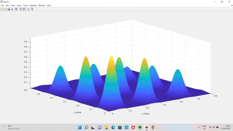
after ending the for loop ,describing the figure 1,
with surf command which gives te 3 dimensional plot
using shading interp gives the smooth surface.
hrnce stating the subplots.
hold on is used to add the second line plot with out deleting the existing one
labelling x & y
hence we get the plot as
hence to better than first study,to increase the size & to get accurate
the same 2 nd case study is carried out with same steps
hence the for loop syntax becomes
for i=1:num_cases
[inputs,fopt(i)]=ga(@stalagmite,2,[],[],[],[],[0;0],[0.6;0.6]);
xopt(i)=inputs(1);
yopt(i)=inputs(2);
end
here xopt & yopt gives the values of xinput & yinput.
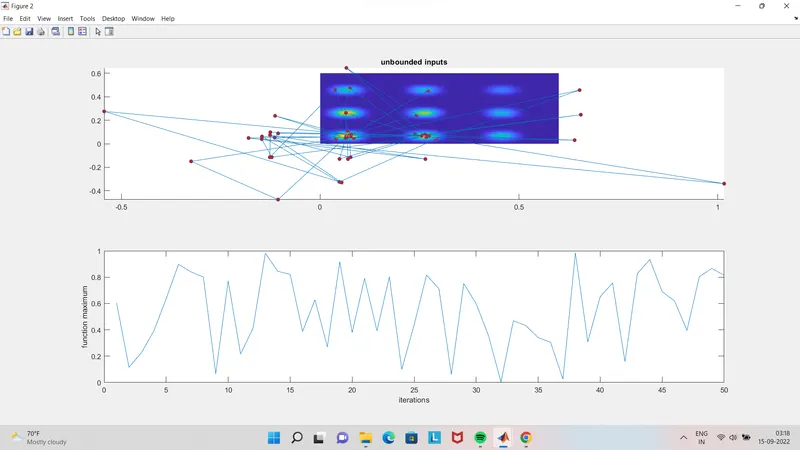
after ending the for loop ,describing the figure 2,
with surf command which gives te 3 dimensional plot
using shading interp gives the smooth surface.
hrnce stating the subplots.
hold on is used to add the second line plot with out deleting the existing one
labelling x & y
unbounded inputs
case 2
to overcome the population size & to increase the global maxima
to get more accurate,we start to calculate case 2
bounded inputs
for loop becomes
for i=1:num_cases
[inputs,fopt(i)]=ga(@stalagmite,2,[],[],[],[],[0;0],[0.6;0.6]);
xopt(i)=inputs(1);
yopt(i)=inputs(2);
end
here xopt(i)& yopt (i)gives the values of xinput & yinput.
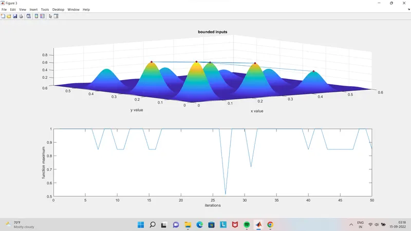
after ending the for loop ,describing the figure 3,
with surf command which gives te 3 dimensional plot
using shading interp gives the smooth surface.
hrnce stating the subplots.
hold on is used to add the second line plot with out deleting the existing one
labelling x & y
hence the bounded input fig 3 is
hence the figure gives the result for bounded lnputs
Toovercome the population size & to increase the global maxima
to get more accurate,we start to calculate case 3
CASE 3 increases the population size
by doing this we are increasing the probability of function
options=optimoptions(ga)
hence he for loop syntax becomes
for i=1:num_cases
[inputs,fopt(i)]=ga(@stalagmite,2,[],[],[],[],[0;0],[0.6;0.6],[],[]);
xopt(i)=inputs(1);
yopt(i)=inputs(2);
bounded inputs
here xopt & yopt gives the values of xinput & yinput.
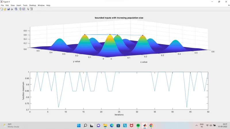
after ending the for loop ,describing the figure 4
with surf command which gives te 3 dimensional plot
using shading interp gives the smooth surface.
hrnce stating the subplots.
hold on is used to add the second line plot with out deleting the existing one
labelling x & y
plot is shown population size & to increase the global maxima
this is how we gwt thw results for 3 cases.
ERRORS FACED
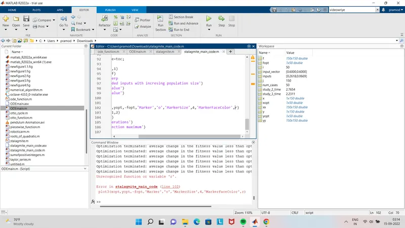
problem-error faced at line 102
solution- wrong usage of comma before marker.after correcting that it solved
ERROR 2
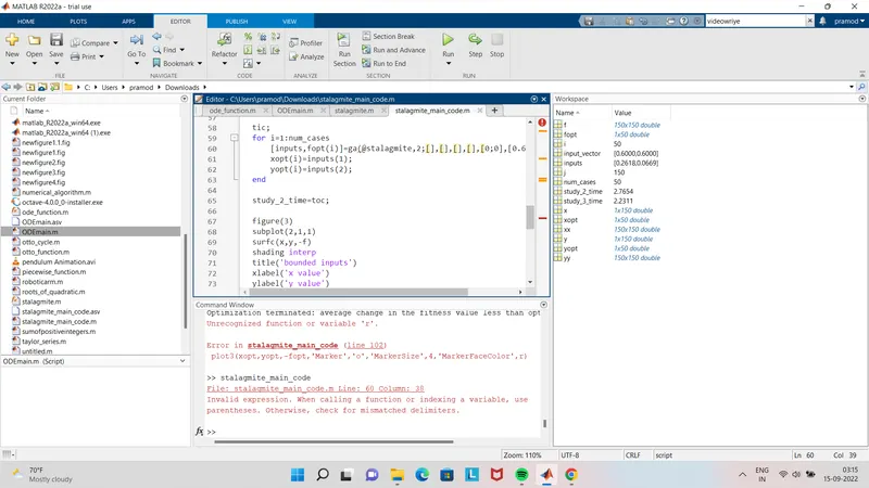
problem-error faced at line 60
solution-instead of using comma i used semicolon for each characters.after correcting it solved.
ERROR 3
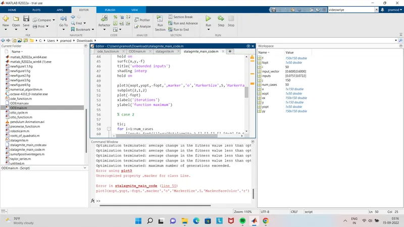
problem;error in plot line
solution;specifing color r is not subjected with single quotes.
'r' after correcting it solved
CONCLUSION
code is written to optimise the stalagmite function and find the global maxima of the function.
All three cases are carriede out & result figures/plots are shown
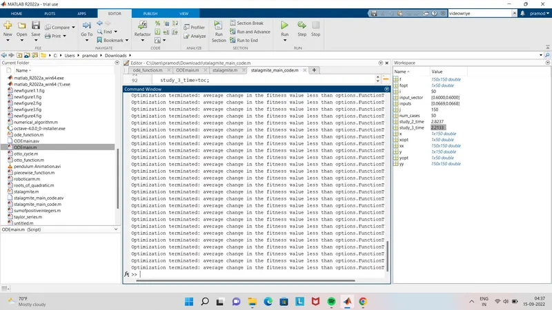
For study 2 time=2.823725400000000
for study 3 time-=2.213334800000000
Results of command window & editor values are displayed
clear all
close all
clc

%input for search space
x=linspace(0,0.6,150);
y=linspace(0,0.6,150);

%use of meshgrid command
[xx,yy]=meshgrid(x,y);

%number of iterations
num_cases=50;

%starting the loop
for i=1:length(xx)
    for j=1:length(yy)
        input_vector(1)=xx(i,j);
        input_vector(2)=yy(i,j);
        f(i,j)=stalagmite(input_vector);
    end
end

figure(1)
surfc(xx,yy,-f)
shading interp
xlabel('x value')
ylabel('y value')

%case 1

for i=1:num_cases
    [inputs,fopt(i)]=ga(@stalagmite,2);
    xopt(i)=inputs(1);
    yopt(i)=inputs(2);


end

%plot the result of study 1

figure(2)
subplot(2,1,1)
hold on
surfc(x,y,-f)
title('unbounded inputs')
shading interp
hold on

plot3(xopt,yopt,-fopt,'marker','o','MarkerSize',5,'MarkerFaceColor','r')
subplot(2,1,2)
plot(-fopt)
xlabel('iterations')
ylabel('function maximum')

% case 2

tic;
for i=1:num_cases
    [inputs,fopt(i)]=ga(@stalagmite,2,[],[],[],[],[0;0],[0.6;0.6]);
    xopt(i)=inputs(1);
    yopt(i)=inputs(2);
end

study_2_time=toc;

figure(3)
subplot(2,1,1)
surfc(x,y,-f)
shading interp
title('bounded inputs')
xlabel('x value')
ylabel('y value')
hold on

plot3(xopt,yopt,-fopt,'marker','o','MarkerSize',5,'MarkerFaceColor','r')
subplot(2,1,2)
plot(-fopt)
xlabel('iterations')
ylabel('function maximum')

%study 3

tic
for i=1:num_cases
    [inputs,fopt(i)]=ga(@stalagmite,2,[],[],[],[],[0;0],[0.6;0.6],[],[]);
    xopt(i)=inputs(1);
    yopt(i)=inputs(2);

end

study_3_time=toc;
figure(4)
subplot(2,1,1)
surfc(x,y,-f)
shading interp
title('bounded inputs with incresing population size')
xlabel('x value')
ylabel('y value')
 hold on

 plot3(xopt,yopt,-fopt,'Marker','o','MarkerSize',4,'MarkerFaceColor','r')
 subplot(2,1,2)
 plot(-fopt)
 xlabel('iterations')
 ylabel('function maximum')


Genetic Algorithm function code


function[f]=stalagmite(input_vector)

a=input_vector(1);
b=input_vector(2);

fx=(sin(5.1*pi*input_vector(1)+0.5))^6;
fy=(sin(5.1*pi*input_vector(2)+0.5))^6;

fxx=exp((-4*log(2)*(((input_vector(1)-0.0667)^2)/0.64)));
fyy=exp((-4*log(2)*(((input_vector(2)-0.0667)^2)/0.64)));

f=-(fx*fy*fxx*fyy);
end