Week 4.1 - Solving second order ODEs

AIM:-Solving second order ODEs

EXPLAINATION::=

some inputs are given

g = gravity in m/s2,

L = length of the pendulum in m,

m = mass of the ball in kg,

b=damping coefficient.

L=1 metre,

m=1 kg,

b=0.05.

g=9.81 m/s2

some function is defined in seperate file

here the name of the function file should be same to the function .

function [dtheta_dt]=ode_function(t,theta,b,g,l,m)

theta1=theta(1);

theta2=theta(2);

dtheta1_dt=theta2;

dtheta2_dt=-(b/m)*theta2-(g/l)*sin(theta1);

dtheta_dt=[dtheta1_dt;dtheta2_dt];

end

here this function file gives the relation b/w inputs

& this function is derived with the following figure

here considering the function we start to write the program ,considering all the inputs stated above

%solve ODE

[t,results]=ode45(@(t,theta) ode_function(t,theta,b,g,l,m),t_span,theta_0);

this equation gives the result for the folloeing ODE

& by substituting all the given input values in the above equation we get some results.

after that ,plotting will be done time vs plot

where time (seconds) along xaxis

plot along y axis

we get the plot like the following figure

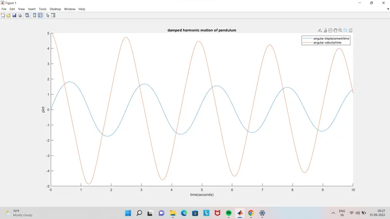
after plotting the figure time vs plot

we use' for ' loop

syntax

for i=1:length(results(:,1))

% origin_points

x0=0;

y0=0;

%max positions

x1=l*sin(results(i,1));

y1=-l*cos(results(i,1));

%plotting

figure(2)

plot([-1 1],[0 0],'LineWidth',5)

hold on

plot([x0 x1],[y0 y1],'linewidth',3)

hold on

plot ([x0 x1],[y0 y1],x1,y1,'g.','MarkerSize',50,'linewidth',2)

axis([-1.5 1.5 -1.5 1.5])

title('animation of transient behaviour of pendulum')

hold off

% grid on

M(ct)=getframe(gcf);

ct=ct+1;

end

here for loop states that for the origin points/ starting points as x0 y0

&

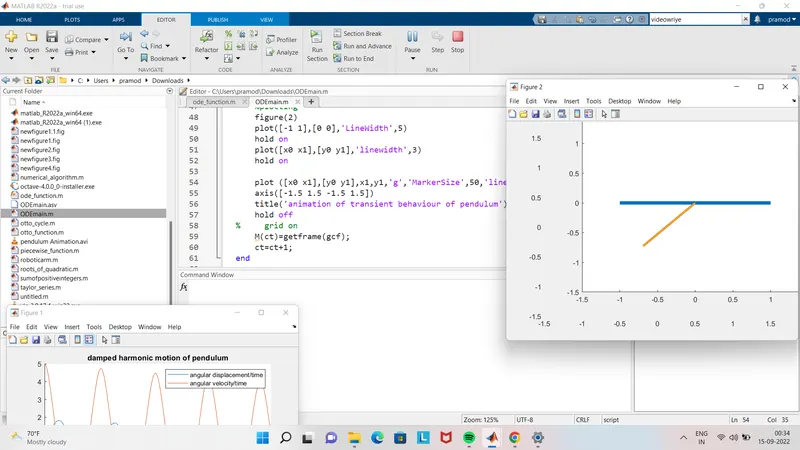
x1=l*sin(results(i,1))

y1=-l*cos(results(i,1)) as a ending points as x1 & y1 .

one end of the pendulum is fixed

for plotting along x axis a x0 y0

yaxis as y0 y1

witha line width of 5

& same plotting

plot ([x0 x1],[y0 y1],x1,y1,'g.','MarkerSize',50,'linewidth',2)

here g. gives the ball structure at the end of pendulum ,marker size stated a s50 making line width 2

getframe is used to get the axis

hence the plot is designed .but to get the animated plot structure

movie(M)

which is done as a movie

videofile=VideoWriter('pendulum Animation.avi','uncompressed avi');

here video file is stated

open(videofile)

writeVideo(videofile,M)

file name is created & that is saved.

hence the Animated video is seen like in the following link

https://youtu.be/akfuxGIJ-28

The youtube link is uploaded as a reference of Animated pendulum working.

Errors faced during the program

error 1

problem-did not get the pendulum end point

solutionOvercoming-After giving "g. " i got the result .

ERROR 2

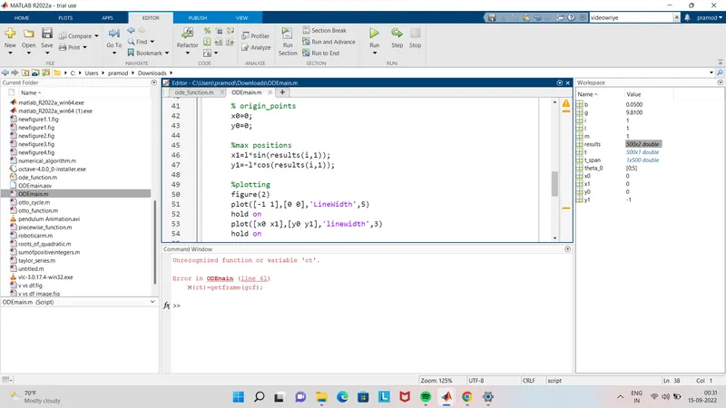
PROBLEM=error facing like this @line 61 .

SOLUTION=missed to state the value fot Ct

after describing Ct=1 ,problem solved.

ERROR 3

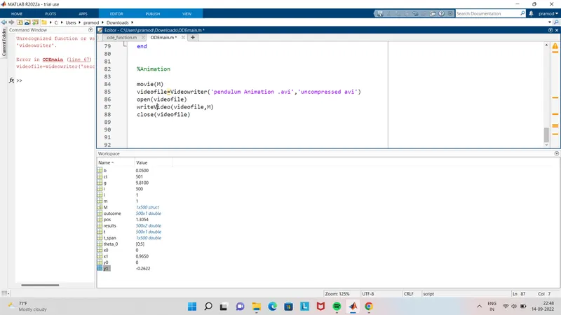
Problem-erroe was facing @line number 87,where it was like

writevideo(videofile,M)

solution- here V was written in small letter,after writing it in caps the problem resolved.

CONCLUSION

Hence

X0=0

Y0=0

X1=0.887596128494767

Y1=-0.460622527326988

1-----THe plot is shown as figure (1)

2-----Animated result is displayed in youtube

https://youtu.be/akfuxGIJ-28

3----Errors faced are displayed & solved.

MAIN ODE PROGRAM



clear all
close all
clc

%Damping coefficient=b
b=0.05;

%gravity=g m/s^2
g=9.81;

%length od pendulum string =l
l=1;

%mass m in kg
m=1;

%Initial condition 
theta_0=[0;5];

%time points
t_span=linspace(0,10,500);

%solve ODE
[t,results]=ode45(@(t,theta) ode_function(t,theta,b,g,l,m),t_span,theta_0);


figure(1)
hold on
plot(t,results(:,1))
plot(t,results(:,2))
title('damped harmonic motion of pendulum')
legend('angular displacement/time','angular velocity/time')
ylabel('plot')
xlabel('time(seconds)')

ct=1; 
for i=1:length(results(:,1))

    % origin_points
    x0=0;
    y0=0;

    %max positions
    x1=l*sin(results(i,1));
    y1=-l*cos(results(i,1));

    %plotting
    figure(2)
    plot([-1 1],[0 0],'LineWidth',5)
    hold on
    plot([x0 x1],[y0 y1],'linewidth',3)
    hold on

    plot ([x0 x1],[y0 y1],x1,y1,'g.','MarkerSize',50,'linewidth',2)
    axis([-1.5 1.5 -1.5 1.5])
    title('animation of transient behaviour of pendulum')
    hold off
%     grid on
    M(ct)=getframe(gcf);
    ct=ct+1;
end



%Animation

movie(M)
videofile=VideoWriter('pendulum Animation.avi','uncompressed avi');
open(videofile)
writeVideo(videofile,M)
close(videofile)







ODE FUNCTION CODE 

function [dtheta_dt]=ode_function(t,theta,b,g,l,m)
theta1=theta(1);
theta2=theta(2);
dtheta1_dt=theta2;
dtheta2_dt=-(b/m)*theta2-(g/l)*sin(theta1);
dtheta_dt=[dtheta1_dt;dtheta2_dt];
end