Week 5 - Genetic Algorithm

%Define Stalagmite Function


function [f] = stalagmite(input_vector)
x = input_vector(1);
y = input_vector(2);
t1 = (sin((5.1*pi*x)+0.5))^6;
t2 = (sin((5.1*pi*y)+0.5))^6;
t3 = exp(-4*log(2)*((x-0.0667)^2)/0.64);
t4 = exp(-4*log(2)*((y-0.0667)^2)/0.64);
f = -(t1*t2*t3*t4);
end

2. Coding for the Genetic Algorithm for this stalagmite functino.

clear all
close all
clc

%Definie our search space
x = linspace(0,0.6,150);         %x array
y = linspace(0,0.6,150);         %y array
n = 50;                          %number of cases

%Creating a 2D mesh
[xx yy] = meshgrid(x,y);

%Evaluating a stalagmite function
for i = 1:length(xx)
    for j = 1:length(yy)
        input_vector(1)=xx(i,j);
        input_vector(2)=yy(i,j);
        f(i,j) = stalagmite(input_vector);
    end
end

%Study 1 : Statistical Behaviour

tic
for i = 1:n
    [inputs,fopt(i)] = ga(@stalagmite,2);
    xopt(i) = inputs(1);
    yopt(i) = inputs(2);
end
study1_time = toc

figure(1)
subplot(2,1,1)
hold on
surfc(xx,yy,-f)
shading interp
xlabel('X-axis')
ylabel('Y-axis')
title('Statistical Behaviour with Unbound inputs')
plot3(xopt,yopt,-fopt,'marker','o','markersize',5,'markerfacecolor','r')
subplot(2,1,2)
plot(-fopt)
xlabel('No. of Iterations')
ylabel('Function maximum')

%Study2 : Statistical behaviour with upper and lower bounds

tic
for i = 1:n
    [inputs,fopt(i)] = ga(@stalagmite,2,[],[],[],[],[0;0],[1;1]);
    xopt(i) = inputs(1);
    yopt(i) = inputs(2);
end
study2_time = toc

figure(2)
subplot(2,1,1)
hold on
surfc(xx,yy,-f)
shading interp
xlabel('X-axis')
ylabel('Y-axis')
title('Statistical behaviour with upper and lower bounds')
plot3(xopt,yopt,-fopt,'marker','o','markersize',5,'markerfacecolor','r')
subplot(2,1,2)
plot(-fopt)
xlabel('No. of Iterations')
ylabel('Function maximum')

%Study3 : Statistical Behaviour with increasing iterations of GA

options = optimoptions('ga');
options = optimoptions(options,'PopulationSize',300);

tic
for i = 1:n
    [inputs,fopt(i)] = ga(@stalagmite,2,[],[],[],[],[0;0],[1;1],[],[],options);
    xopt(i) = inputs(1);
    yopt(i) = inputs(2);
end
study3_time = toc

figure(3)
subplot(2,1,1)
hold on
surfc(xx,yy,-f)
shading interp
xlabel('X-axis')
ylabel('Y-axis')
title('Statistical Behaviour with increasing iterations')
plot3(xopt,yopt,-fopt,'marker','o','markersize',5,'markerfacecolor','r')
subplot(2,1,2)
plot(-fopt)
xlabel('No. of Iterations')
ylabel('Function maximum')

 3. Output with Srceenshot.

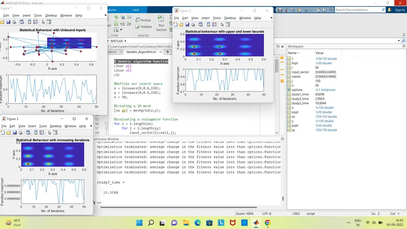
•  Plots of the output

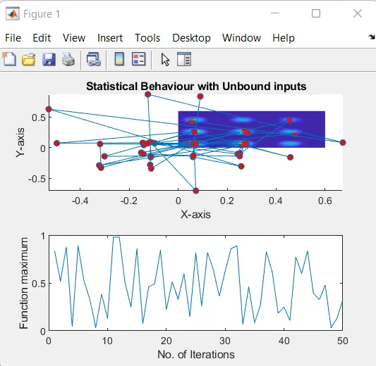
1. Statistical Behaviour with unbound inputs.

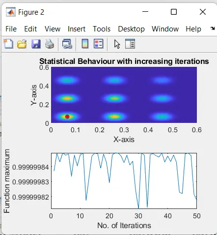
2. Statistical Behaviour with increasing iterations

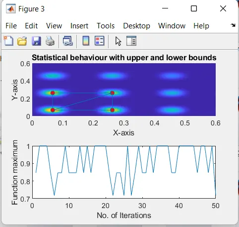
3. Statistical Behaviour with upper and lower Bounds 

4. Step-wise explanation of your code.

• The code starts with clear all, close all and clc where, ‘clear all’ command is used to clear the data stored in the workspace, ‘close all’ command is used to close all plots and figures, ‘clc’ command is used to clear the command window.
• Then the ‘x’ array and ‘y’ array is defined using ‘linspace’ command to create values at 150 equal intervals.
• A 2D mesh of x and y array is created by using ‘meshgrid’ command and the number of iterations or cases that the code should perform is defined. This is given by n = 50.
• To evaluate the stalagmite function, ‘for’ loop is used where ‘i’ is initialized and for every value of ‘i’ another ‘for’ loop is used to initialize ‘j’.
• The input vector values of ‘xx’ and ‘yy’ are defined and the stalagmite function for these input vector is defined. This will form a basic stalagmite function and we can plot it separately if needed.
• After preparing the inputs needed for the function, next step is to obtain the results for 3 cases of the genetic algorithm. In first case or study, the maximum value of function is found out with no restrictions, no bounds and no limits.
• This is done using ‘for’ loop where we use ‘ga’ syntax to give values for inputs and optimum max value. The stalagmite function is called in ‘ga’ syntax and number of variables ‘nvars’ are 2.
• To know the time that is taken to solve the loop for 50 iterations, ‘tic’ and ‘toc’ command is used before and after the loop respectively.
• Then the function created in the loop is plotted by using ‘surfc’ command for ‘xx, yy and function output’. To neglect the gridlines on the surface and obtain a smooth and clean plot, ‘shading interp’ command is used. The ‘subplot(2,1,1)’ is used to plot multiple plots on same figure which also divides figure in grid of 2x1 and axes to be placed at 1.
• The ‘plot3’ command plots the 3D points at ‘xopt, yopt and optimum value of function’ with ‘o’ shaped and red colour. The labels and title are then provided. Now in the same figure, the values of optimum function ‘fopt’ are plotted for 50 iterations.
• The results of the above case will be different for each time we run the program. To get same value each time, we need to restrict the program within specific bounds namely upper bound and lower bound. The procedure for coding and plottind this procedure is same as Study 1. The only difference is in the ‘ga’ syntax. This time the algorithm is provided lower limits and upper limits as [0;0] and [1;1] respectively.
• After plotting the results for Study 2 or the bounded case, it is observed that the results are not same every time the program terminates. A solution to this problem is to increase the number of cases or iterations.
• So for Study 3, the number of iterations are increased to 300. So for this study, the syntax, “options = optimoptions(‘SolverName’,’Name’,‘Value’)” is used which returns with named parameter ‘Populations’ with the altered values ‘300’.
• The syntax for ‘ga’ contains ‘option’ term and the rest of the code is same as for Study 1 and 2.

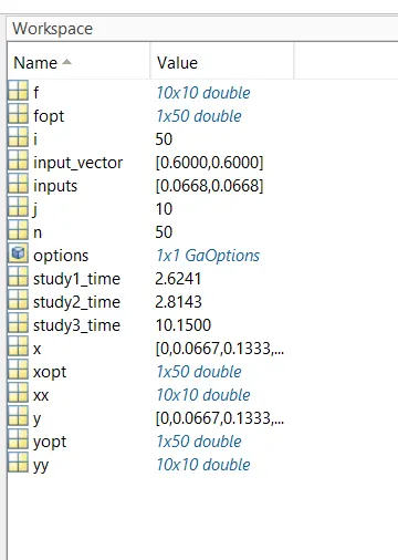
5. Workspace Values 

•  Google Drive Link for Folders

https://drive.google.com/drive/folders/15aN7WKPcxR6e-lIJCduMHqSTu6KDodQZ?usp=sharing

•  REFERENCES :

1. https://in.mathworks.com/help/gads/genetic-algorithm-options.html
2. https://in.mathworks.com/help/gads/genetic-algorithm.html
3. https://in.mathworks.com/help/gads/some-genetic-algorithm-terminology.html