Week 5 - Genetic Algorithm

AIM

Write a code in MATLAB to optimize the stalagmite function and find the Global Maxima of the function.

GENETIC ALGORITHM

Genetic Algorithms are a method that work based on Darwin’s theory of natural selection

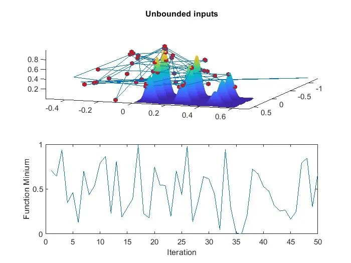
The fittest survives, and has a greater chance of breeding and passing forward its genetic information.

Let’s say we have an equation unsolvable by analytical methods, or an optimisation problem that takes too long to solve.

First, the program randomly generates a population of solutions.

Then, these solutions are evaluated by a function adequate to the problem, determining how well they ‘fit’.

The ones with the best fit will have a greater chance of being selected to breed and generate the next population.

Finally, the selected solutions are recombined amongst themselves creating a new population.

Random shifts, just like mutations, also happen in order to introduce more variability.

Whereas the first generation was completely random, the second is biased towards solutions with better results.

After several iterations, they tend to converge to the optimum value.

In essence, it is very close to what evolution proposes.

A population is evaluated by the environment the fittest have a greater chance to breed and pass their ‘good’ genes along, which will then be recombined and mixed.

The next generation will now have more of the genetic characteristics that represent a good fit in the current environment.

GA’s are especially attractive to rapidly find solutions to difficult high-dimension problems, with little information about the search space.

As a downside, it does not always return the optimal value, as any heuristic.

Instead, it returns a value as good as the problem and the stopping criteria permit.

Selection rules - Select the individuals, called parents that contribute the population at the next generation.

Crossover rules - Combine two parents to from children for the next generation.

Mutation rules - Apply random changes to individual parents to from the children.

Genetic Algorithms are primarily used in optimization problems of various kinds, but they are frequently used in other application areas as well.

The areas in which Genetic Algorithm are frequently used are listed below.

Optimization – Genetic algorithm are most commonly used in optimization problem wherein we have to maximize or minimize a given objective function values under given set of constraints.

Economics – GAs are used to characterize various economic model like the cobweb model, game theory equilibrium resolution, asset pricing, etc.

Neutral Network – GAs are used to train neutral network, particularly recurrent neural networks.

Image Processing – GAs are used for various digital image processing(DIP) takes as well as dense pixel matching.

The above are same of the areas where the genetic algorithm is extensively used for optimization.

Fitness Function – The fitness function takes the solution as input and produces the suitability of the solution as the output. The evaluates how close the solution is to the optimal solution of the desired problem.

The Syntax for GA in Matlab

x = ga(fun,nvars,A,b,Aeq,beq,lb,ub,nonlcon,intcon,options)

The Syntax is explained as follows -

‘x’ is the variable to store the output of the genetic algorithm.

‘fun’ is the function handle to call the function.

‘A’ and ‘b’ are used to represent the linear inequalities of the function, if the linear inequalities do not exist, they can be set as empty [].

‘Aeq’ and ‘beq’ are used to represent the equality constraints. Similarly, if the linear equalities do not exits, they can be set as empty [].

‘lb’ and ‘ub’ are used to simplify the upper and the lower bounds of the variables of the function.

‘nonlcon’ represents the non-linear constraints.

‘intcon’ represent the integer constraint, such that the value of the function is an integer.

‘options’ used to provide the value of the default parameters used named parameters, if it is required to replace the default parameters. This is done by using the ‘optimoptions’.

CODE

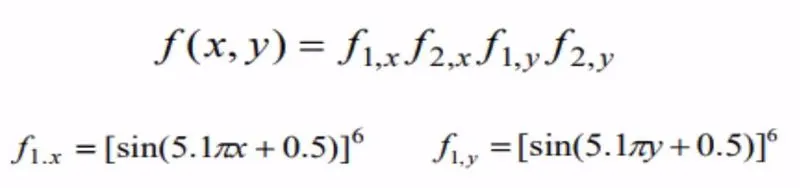
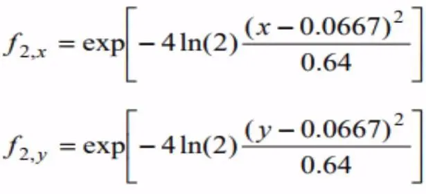
The following is the given stalagmite function for which we need to find the global maxima.

clear
close
clc
  
x = linspace(0,0.6,150);
y = linspace(0,0.6,150);

% Creating a 2Dimensional mesh
[xx ,yy] = meshgrid(x,y);

% Evaluating the Stalagmite Function
for i = 1:length(xx)
    for j = 1:length(yy)
        input_vector(1)=xx(i,j);
        input_vector(2)=yy(i,j);
       
        f(i,j) = stalagmite(input_vector);               

    end
end


surfc(xx,yy,f)
xlabel('x value')
ylabel('y value')

hold on
shading interp

[x,fval] = ga(@stalagmite, 2)

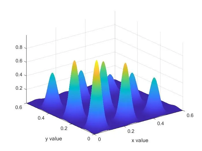
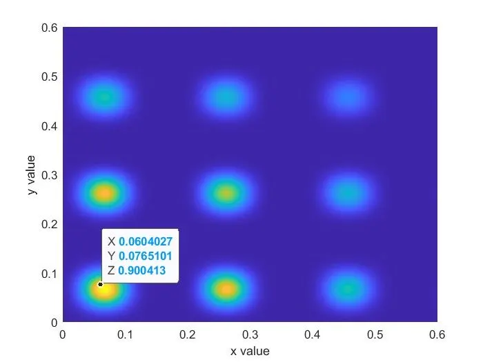
MATLAB code to optimize the stalagmite function and find the Global Maxima of the function

CODE

% Defining Our Search Space
x = linspace(0,0.6,150);
y = linspace(0,0.6,150);
num_cases = 50                                            % no of itration

%% Creating a 2Dimensional mesh
[xx ,yy] = meshgrid(x,y);

% Evaluating the Stalagmite Function
for i = 1:length(xx)
    for j = 1:length(yy)
        input_vector(1)=xx(i,j);
        input_vector(2)=yy(i,j);
        input_vector=[input_vector(1),input_vector(2)];
        GA(i,j) = stalagmite(input_vector);               
    end
end


% Study-1 | Statistical Behaviour | In Unbounded condition

                                                  

%tic_toc command for calculating the itration time
tic 
for i = 1:num_cases
        [input, GA_opt(i)] = ga(@stalagmite,2);
        xopt(i) = input(1);
        yopt(i) = input(2);
end

study_1_time = toc

%Plotting the Graph
figure(1) 
subplot(2,1,1)
hold on
surfc(x,y,-GA)
shading interp
plot3(xopt,yopt,-GA_opt,'marker','o','markersize',5,'markerfacecolor','r')
title('Unbounded inputs')
subplot(2,1,2)
plot(-GA_opt)
xlabel('Iteration')
ylabel('Function Minium')


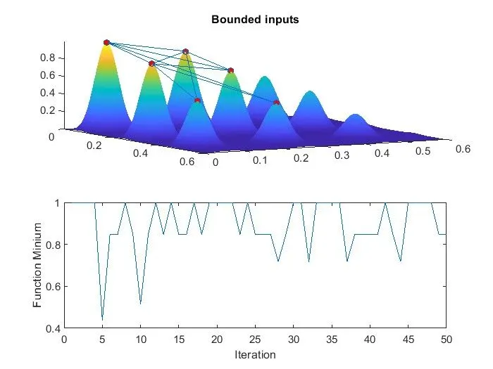
% Study-2 | Statistical behaviour - with upper & lower bounds
                              
%tic_toc command for calculating the itration time
tic
for i = 1:num_cases
    [input, GA_opt(i)] = ga(@stalagmite,2,[],[],[],[],[0;0],[1;1]);
        xopt(i) = input(1);
        yopt(i) = input(2);
end
study_2_time = toc

%Plotting the Graph
figure(2)
subplot(2,1,1)
hold on
surfc(x,y,-GA)
shading interp
plot3(xopt,yopt,-GA_opt,'marker','o','markersize',5,'markerfacecolor','r')
title('Bounded inputs')
subplot(2,1,2)
plot(-GA_opt)
xlabel('Iteration')
ylabel('Function Minium')


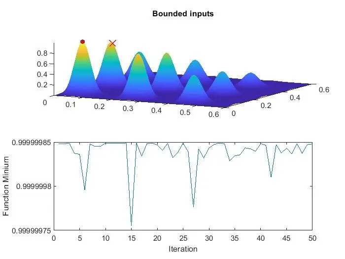
% Study-3 | Increasing GA Iterations

%Calculating the optimum solution for 'ga' and save in options(variable)
options = optimoptions('ga');                
%increasing the size of population
options = optimoptions(options,'PopulationSize',240);      

%tic_toc command for calculating the itration time
tic                                                        
for i = 1:num_cases
    [input, GA_opt(i)] = ga(@stalagmite,2,[],[],[],[],[0;0],[1;1],[],[],options);
        xopt(i) = input(1);
        yopt(i) = input(2);
end
study_3_time = toc

%Plotting the Graph
figure(3)
subplot(2,1,1)
hold on
surfc(x,y,-GA)
shading interp
plot3(xopt,yopt,-GA_opt,'marker','o','markersize',5,'markerfacecolor','r')
title('Bounded inputs')
subplot(2,1,2)
plot(-GA_opt)
xlabel('Iteration')
ylabel('Function Minium')

STALAGMITE CODE

function [GA] = stalagmite(input_vector)

x=input_vector(1);
y=input_vector(2);


term1 = pi*5.1*x;
term2 = pi*5.1*y;
term3 = ((x-0.0667)^2/0.64);
term4 = ((y-0.0667)^2/0.64);
term5 = (-4)*log(2);

xf1 = (sin(term1 + 0.5)).^6;

yf1 = (sin(term2 + 0.5)).^6;

xf2 = exp(term5*term3);

yf2 = exp(term5*term4);



GA=-(xf1*yf1*xf2*yf2);

end

Statistical Behaviour

WITH UPPER AND LOWER BOUNDS

INCREASING GA ITERATIONS

Step 1: Clearing workspace, command window & closing all plots

Step 2: Define our search space by using linspace command

Step 3: Calculating a 2 Dimentionl mesh using meshgrid command

Step 4: Evaluating the stalagmite function for each value of x & y

Step 5: using GA command with unbounded inputs means optimum value may be come from outside of search space, Refer attached graph.

Step 6: using GA command with bounded inputs means optimum value will be come from inside of search space, Refer attached graph. However there will be huge variation in optimum value.

Step 7: using GA command with bounded inputs means optimum value will be come from inside of search space, Refer attached graph. However this time to avoid huge variation in optimum value, we have increased initial population size to 200. ( If we do not specify initial population in program, MATLAB take 50 as initial population)

Syntax for ga- ga(@stalagmite,2,[ ],[ ],[ ],[ ],[0;0],[1;1],[ ],[ ],options)

ga - To find the minimum of function using Genetic Algorithm
fun - finds a local minimum to function
nvars - number of variables.
A - Linear Inequality Constraints,specified as a real matrix
b - Linear Inequality Constraints,specified as a real vector
Aeq - Linear equality Constraints,specified as a real matrix
beq - Linear equality Constraints,specified as a real matrix
lb - Lower Bound
ub- Upper Bound
nonlcon - Nonlinear Constraints, specified as function handle
options- Optimization options, specified as the output

We do Multiple iteration is to get the Global maxima in desired range. The main motive of doing so is to get the only 1 desired optimum output which is required for given problem.

CONCLUSION

code in MATLAB to optimise the stalagmite function and find the global maxima of the function, the concept of genetic algorithm, Plot graphs for all 3 studies are shown above.