Week 5 - Genetic Algorithm

Report

MAIN CODE

clear all 
close all
clc

n=150;
x = linspace(0,0.6,150);
y = linspace(0,0.6,150);

%creating two dimensional grid
[xx, yy] = meshgrid(x,y);
tic
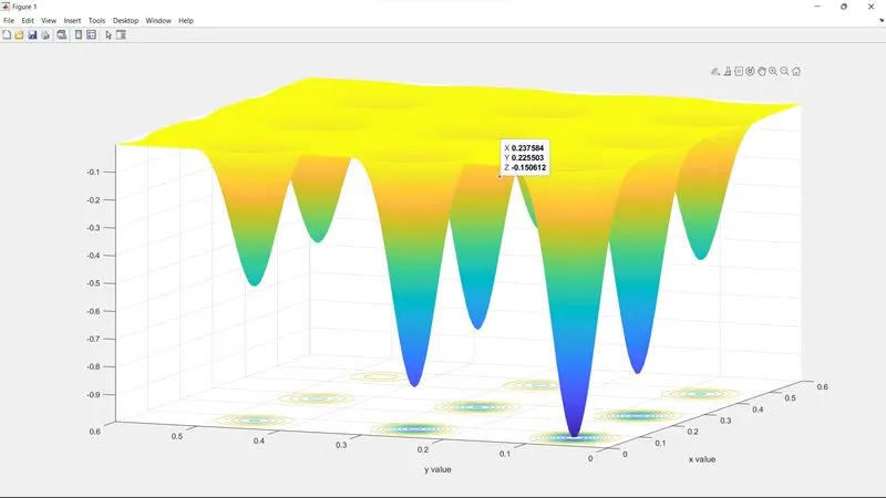
%evaluating the stalagmite function

for i = 1:length(xx)
    for j = 1:length(yy)
        input_vector(1)= xx(i,j);
        input_vector(2)= yy(i,j);
        f(i,j) = stalagmite(input_vector);
    end
end

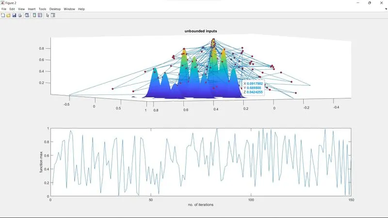
%case 1 (unbounded inputs)

tic
for i = 1:n
    [inputs,fopt(i)]= ga(@stalagmite, 2);
    xopt(i)=inputs(1);
    yopt(i)=inputs(2);
end

figure(2)
subplot(2,1,1)
hold on
surfc (x,y,-f)
shading interp
plot3(xopt,yopt,-fopt,'marker','o','markersize',5,'markerfacecolor','r')
title('unbounded inputs')
subplot(2,1,2)
plot(-fopt)
xlabel('no. of iterations');
ylabel('function max');

study_time1=toc;


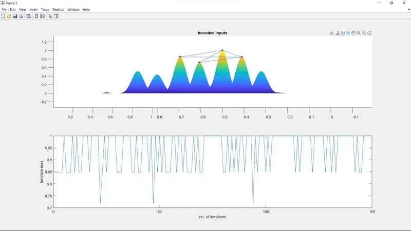
% second case (bounded inputs)

tic
for i = 1:n
    [inputs,fopt(i)]= ga(@stalagmite, 2,[],[],[],[],[0;0],[0.6;0.6]);
    xopt(i)=inputs(1);
    yopt(i)=inputs(2);
end

figure(3)
subplot(2,1,1)
hold on
surfc (x,y,-f)
shading interp
plot3(xopt,yopt,-fopt,'marker','o','markersize',5,'markerfacecolor','r')
title('bounded inputs')
subplot(2,1,2)
plot(-fopt)
xlabel('no. of iterations');
ylabel('function max');

study_time2=toc;


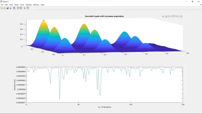
% third case (bounded inputs with increased population)

tic
options=optimoptions('ga');
options=optimoptions(options,'PopulationSize',500);

for i = 1:n
    [inputs,fopt(i)]= ga(@stalagmite,2,[],[],[],[],[0;0],[1;1],[],[],options);
    xopt(i)=inputs(1);
    yopt(i)=inputs(2);
end

figure(4)
subplot(2,1,1)
hold on
surfc (x,y,-f)
shading interp
plot3(xopt,yopt,-fopt,'marker','o','markersize',5,'markerfacecolor','r')
title('bounded inputs with increases population')
subplot(2,1,2)
plot(-fopt)
xlabel('no. of iterations');
ylabel('function max');

study_time3=toc;

FUNCTION CODE  (stalagmite)

function [f] = stalagmite(input_vector)
f1x = (sin((5.1*pi).*input_vector(1)+0.5)).^6;
f1y = (sin((5.1*pi).*input_vector(2)+0.5)).^6;

f2x = exp((((input_vector(1)-0.0667).^2)/0.64).*(-4*log(2)));
f2y = exp((((input_vector(2)-0.0667).^2)/0.64).*(-4*log(2)));
f1=f1x*f1y*f2x*f2y;
f=-f1;
end

Errors occured

No errors were occured during this as the whole conceptnwas cleared durimng several one one one sessions.

2. Genetic Algorithms are search based algorithms based on the concepts of natural selection and genetics.A genetic algorithm is a natural process that is used for the selection of the fittest individuals. The main use of the genetic algorithm is for reproduction to produce offspring of the next generation, this process of selecting and reproducing the fittest individual is inspired by Charles Darwin’s and named it the "Theory of evolution". Genetic Algorithms are a subset of a much larger branch of computation known as Evolutionary Computation.

Five phases are considered in a genetic algorithm. They are

Initial population
Fitness function
Selection
Crossover
Mutation

Syntax of GA

EXPLANATION

x = ga(fun,nvars) finds a local unconstrained minimum, x, to the objective function, fun. nvars is the dimension (number of design variables) of fun.

x = ga(fun,nvars,A,b) finds a local minimum x to fun, subject to the linear inequalities A*x ≤ b. ga evaluates the matrix product A*x as if x is transposed (A*x').

x = ga(fun,nvars,A,b,Aeq,beq) finds a local minimum x to fun, subject to the linear equalities Aeq*x = beq and A*x ≤ b. (Set A=[] and b=[] if no linear inequalities exist.) ga evaluates the matrix product Aeq*x as if x is transposed (Aeq*x').

x = ga(fun,nvars,A,b,Aeq,beq,lb,ub) defines a set of lower and upper bounds on the design variables, x, so that a solution is found in the range lb ≤ x ≤ ub. (Set Aeq=[] and beq=[] if no linear equalities exist.)

x = ga(fun,nvars,A,b,Aeq,beq,lb,ub,nonlcon) subjects the minimization to the constraints defined in nonlcon. The function nonlcon accepts x and returns vectors C and Ceq, representing the nonlinear inequalities and equalities respectively. ga minimizes the fun such that C(x) ≤ 0 and Ceq(x) = 0. (Set lb=[] and ub=[] if no bounds exist.)

x = ga(fun,nvars,A,b,Aeq,beq,lb,ub,nonlcon,options)

minimizes with the default optimization parameters replaced by values in options. (Set nonlcon=[] if no nonlinear constraints exist.) Create options using optimoptions.

x = ga(fun,nvars,A,b,Aeq,beq,lb,ub,nonlcon,intcon) or

x = ga(fun,nvars,A,b,Aeq,beq,lb,ub,nonlcon,intcon,options) requires that the variables listed in intcon take integer values