Project 2 - Rankine cycle Simulator

Screenrecording of the matlab window is uploded with this.

Main Code

clear all 
close all 
clc

% Rankine Cycle Simulator
disp(' Rankine Cycle');
disp('1-2 is Isentropic Expansion in Turbine\n');
disp('2-3 is constant pressure heat removal\n');
disp('3-4 is Isentropic Compression in Pump\n' );
disp('4-1 Constant pressure Heat addition in Boiler\n');

% Entering the input data for calculation of state points
p1 = input('P1 = ');        %Pressure at Turbine Inlet
T1 = input('T1 = ');       %Temperature at Turbine Inlet
p2 = input('P2 = ');      %Pressure at Condenser


% Taking data from Xsteam file for State point 1
h1 = XSteam('h_pT',p1,T1);        % Enthaply at pressure and Temp 1
s1 = XSteam('s_pT',p1,T1);        % Entropy at pressure and Temp 1


% Taking data from Xsteam file for State point 2
s2 = s1;                            % Because of Isentropic Expansion
sf2 = XSteam('sL_p',p2);           % Saturated liquid entropy at pressure 2
sg2 = XSteam('sV_p',p2);           % Saturated vapour entropy at pressure 2
x2 = (s2-sf2)/(sg2-sf2);            % Vapour Fraction at state point 2
hf2 = XSteam('hL_p',p2);           % Saturated liquid Enthalpy at pressure 2
hg2 = XSteam('hV_p',p2);           % Saturated vapour Enthalpy at pressure 2
h2 = hf2 + (x2*(hg2-hf2));          % Enthalpy at state point 2

% Taking data from Xsteam file for state point 3
p3 = p2;                            % Constant Pressure heat removal process
s3 = XSteam('sL_p',p3);            % Saturated liquid entropy at Pressure 3
h3 = XSteam('hL_p',p3);            % Saturated liquid Enthalpy at Pressure 3

% Taking data from Xsteam file for State point 4
s4 = s3;                            % Isentropic Compression process
p4 = p1;                            % Constant Pressure heat rejection

% Work done in Turbine for the rankine cycle
W_T = h1-h2;

% Work done required for pump
v3 = XSteam('vL_p',p3);             % Saturated Liquid Vapour at pressure 3
W_P = v3*(p4-p3)*100;               % Work done for pump
h4 = h3 - W_P;                      % Enthalpy at State point 4

% Net work done for Rankine Cycle
W_net = W_T - W_P;

% Heat Addition to System
Q_in = h1-h4;

% Heat Rejection from System
Q_out = h2-h3;

% Thermal Efficiency of Rankine Cycle
T_eff = (W_net/Q_in)*100;

%specific steam consumption  = (Mass flow rate / Net work done)
Sp_S = (3600/W_net);

% Calculation of Temperature at All state Point 2, 3 and 4
T3 = XSteam('Tsat_p',p3);           % Saturation Temperature at Pressure 3
T2 = T3;                            % Becuase of Constant Pressure Heat addition
Cp4 = XSteam('Cp_ps',p4,s4);        % Specific isobaric heat capacity
Cv4 = XSteam('Cv_ps',p4,s4);        % Specific isochoric heat capacity
k = Cp4/Cv4;
T4 = T3/((p3/p4)^((k-1)/k));        % Temperature at State point 4

% Calculation of Other constant for saturated liquid and Vapour
T6 = XSteam('Tsat_p',p1);          % Saturated Temperature at Pressure 1
s5 = XSteam('sL_p',p1);            % Saturated Liquid entropy at pressure 1
s6 = XSteam('sV_p',p1);            % Saturated Vapour entropy at Pressure 1
h5 = XSteam('hL_p',p1);            % Saturated Liquid Enthalpy at Pressure 1
h6 = XSteam('hV_p',p1);            % Saturated Vapour Enthalpy at pressure 1
T5 = T6;

%Plotting for Saturation Line
T = linspace(1,560,1000);
for i = 1:length(T)
    sf(i) = XSteam('sL_T',T(i));   % Saturated Liquid Entropy
    sg(i) = XSteam('sV_T',T(i));   % Saturated Vapour Entropy
    hf(i) = XSteam('hL_T',T(i));   % Saturated Liquid Enthalpy
    hg(i) = XSteam('hV_T',T(i));   % Saturated Vapour Enthalpy
    
end
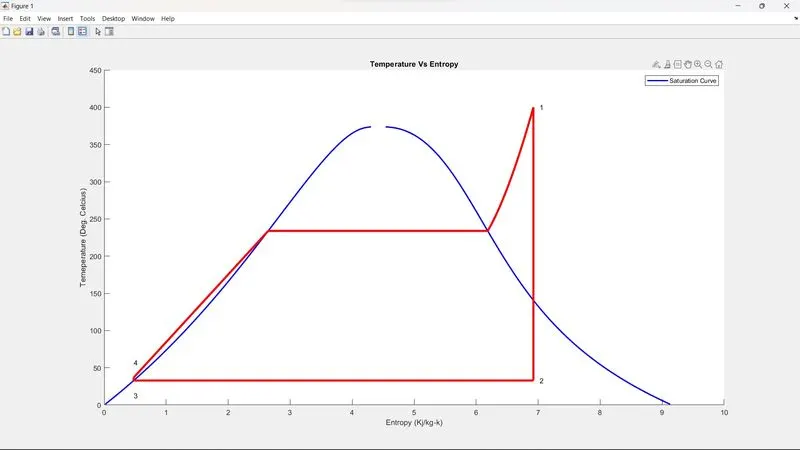
% Plotting T-S Diagram for Rankine Cycle
figure(1)
hold on
plot(sf,T,'color','b','linewidth',2)
plot(sg,T,'color','b','linewidth',2)
plot([s1 s2],[T1 T2], 'color', 'r', 'linewidth',3)
plot([s2 s3],[T2 T3], 'color', 'r', 'linewidth',3)
plot([s3 s4],[T3 T4], 'color', 'r', 'linewidth',3)
plot([s4 s5],[T4 T5], 'color', 'r', 'linewidth',3)
plot([s5 s6],[T5 T6], 'color', 'r', 'linewidth',3)
s_1 = linspace(s6,s1,1000);
for j = 1:length(s_1)
    Tc(j) = XSteam('T_ps',p1,s_1(j));
end
plot(s_1,Tc,'color','r','linewidth',3)
text(s1+0.1, T1, '1')
text(s2+0.1, T2, '2')
text(s3, T3-20, '3')
text(s4, T4+20, '4')
title('Temperature Vs Entropy')
xlabel('Entropy (Kj/kg-k)')
ylabel('Temeperature (Deg. Celcius)')
legend('Saturation Curve')

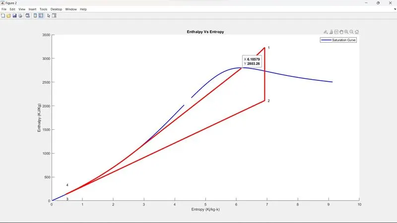
% Plotting H-S Diagram for Rankine Cycle
figure(2)
hold on
plot(sf,hf,'color','b','linewidth',2)
plot(sg,hg,'color','b','linewidth',2)
plot([s1 s2],[h1 h2],'color','r','linewidth',3)
plot([s2 s3],[h2 h3],'color','r','linewidth',3)
plot([s3 s4],[h3 h4],'color','r','linewidth',3)
hc = linspace(h4,h5,100);
for k = 1:length(hc)
    s_c(k) = XSteam('s_ph',p1,hc(k));
end
plot(s_c,hc,'color','r','linewidth',3)
plot([s5 s6],[h5 h6],'color','r','linewidth',3)
for l = 1:length(s_1)
    h_c(l) = XSteam('h_ps',p1,s_1(l));
end
plot(s_1,h_c,'color','r','linewidth',3)
text(s1+0.1,h1,'1')
text(s2+0.1,h2,'2')
text(s3,h3-100,'3')
text(s4,h4+200,'4')
title('Enthalpy Vs Entropy')
xlabel('Entropy (Kj/kg-k)')
ylabel('Enthalpy (KJ/Kg)')
legend('Saturation Curve')

% Displaying Results in Command window
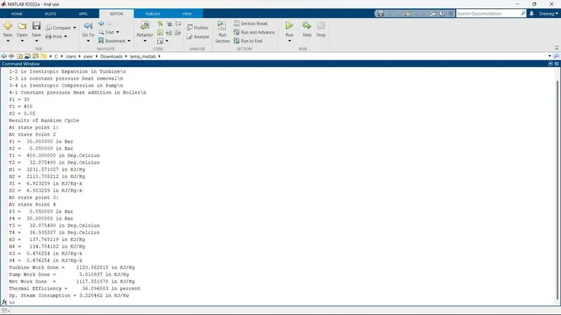
disp('Results of Rankine Cycle')
fprintf('At state point 1:\n')
fprintf('At state Point 2\n')
fprintf('P1 = %10f in Bar\n',p1);
fprintf('P2 = %10f in Bar\n',p2);
fprintf('T1 = %11f in Deg.Celcius\n',T1);
fprintf('T2 = %11f in Deg.Celcius\n',T2);
fprintf('H1 = %12f in KJ/Kg\n',h1);
fprintf('H2 = %12f in KJ/Kg\n',h2);
fprintf('S1 = %9f in KJ/Kg-k\n',s1);
fprintf('S2 = %9f in KJ/Kg-k\n',s2);
fprintf('At state point 3:\n')
fprintf('At state Point 4\n')
fprintf('P3 = %10f in Bar\n',p3);
fprintf('P4 = %10f in Bar\n',p4);
fprintf('T3 = %11f in Deg.Celcius\n',T3);
fprintf('T4 = %11f in Deg.Celcius\n',T4);
fprintf('H3 = %12f in KJ/Kg\n',h3);
fprintf('H4 = %12f in KJ/Kg\n',h4);
fprintf('S3 = %9f in KJ/Kg-k\n',s3);
fprintf('S4 = %9f in KJ/Kg-k\n',s4);
fprintf('Turbine Work Done = %14f in KJ/Kg\n',W_T)
fprintf('Pump Work Done = %15f in KJ/Kg\n',W_P)
fprintf('Net Work Done  = %17f in KJ/Kg\n',W_net)
fprintf('Thermal Efficiency = %13f in percent\n',T_eff)
fprintf('Sp. Steam Consumption = %f in KJ/Kw\n',Sp_S)

STEPWISE EXPLANATION

1. The Rankine cycle process is displayed in the command window and then input variables are entered
2. Then we are using XSteam function file for reading state point. First, we get the value of enthalpy and entropy at state point 1 from the XSteam function file.
3. As process from 1-2 is isentropic compression the entropy at point 1 is equal to point 2.
4. The term ‘sg’ and ‘sf’ are referred to saturated liquid and saturated vapor entropy respectively. This value is used to calculate other function according to mathematical relations.
5. Similarly, other points are taken from XSteam function file which are necessary to calculate other parameters. Work done in turbine and pump are calculated.
6. After calculating the net work done the efficiency of the Rankine cycle is calculated along with specific steam consumption.
7. Then temperature at each point of cycle is calculated using input taken from start of the program and data taken from XSteam file. For given temperature range from lower to higher entropy points are calculated to create the T-S plot. Similarly, another for loop is used to create the saturation curve in each plot.
8. Then plotting is done respectively for T-s and H-s graph in Rankine cycl.

ERRORS

No errors occured.

GRAPH

Output