Week 5 - Genetic Algorithm
AIM
to write a code in MATLAB to optimize the stalagmite function using genetic algorithm and find the global maxima of the function.
GENETIC ALGORITHM
A genetic algorithm (GA) is a computational optimization technique that uses principles of genetic and natural selection to solve optimization and search problems. GAs is a type of evolutionary algorithm that repeatedly modifies a population of potential solutions or individuals over a generation until an optimal solution is reached.
STEPS IN GENETIC ALGORITHM
Initial Population
A random population of individuals is created to represent potential solutions to the problem.
Selection
Individuals are evaluated based on a fitness function that measures how well each solution solves the problem.
Crossover
The top individuals are selected and then crossed over to new individuals.
Mutation
random mutations are introduced to give the individuals special traits.
Repeat
The process is repeated with the new population and the population evolves towards an optimal solution for successive generations.
GAs use biologically inspired operators like mutation, crossover, and selection. They can be used to solve a variety of problems, including optimization decision trees, solving sudoku puzzles, and hyperparameter optimization.
SYNTAX OF ‘GA’ IN MATLAB
[x, fval] = ga(fun, nvars)
[x, fval] = ga(fun, nvars, A, b, Aeq, beq, lb, ub)
[x, fval] = ga(fun, nvars, A, b, Aeq, beq, lb, ub, nonlcon, options)
Parameters
Fun: A function handle to the objective function that you want to minimize.
Nvars: The number of variables in the objective function.
A, b: (optional) Matrices for linear inequality constraints.
Aeq, Beq: (optional) Matrices for linear equality constraints.
LB, UB: (optional) Vectors of lower and upper bounds on the variables respectively.
nonlcon: (optional) A function handle for nonlinear constraint function.
Options: (Optional) A structure created using ‘optimoptions’ to specify options for the genetic algorithm such as population size, crossover fraction, mutation rate, etc.
STEP BY STEP EXPALANTION
Defining The Search Space
x = linspace(0,0.6,150);
y = linspace(0,0.6,150);
num_cases = 50;
‘linspace (0, 0.6, 150)’ generates 150 linearly spaced points between 0 and 0.6 for both ‘x’ and ‘y’.
‘num_cases = 50’ number of iterations.
Creating A 2D Mesh
[xx, yy] = meshgrid(x, y);
‘meshgrid(x,y)’ creates a 2D grid of ‘x’ and ‘y’ values.
Evaluating The Stalagmite Function
tic
for i = 1:length(xx)
for j = 1:length(yy)
input_vector(1) = xx(i,j);
input_vector(2) = yy(i,j);
f(i,j) = stalagmite(input_vector);
end
end
Using the ‘for-loop’ command evaluates the stalagmite functions at each point.
‘tic’ and ‘toc’ are used to record the elapsed time.
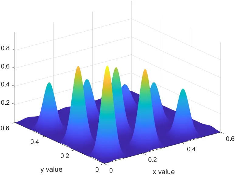
Plotting The Stalagmite Function
figure(1)
surfc(xx,yy,-f);
xlabel('x value')
ylabel('y value')
shading interp
study_time = toc;
‘surfc’ plots a 3D surface plot.
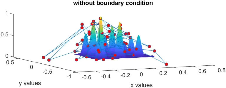
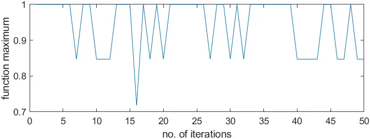
Study One : GA Without Boundary Conditions
tic
for i = 1:num_cases
[inputs, fopt(i)] = ga(@stalagmite,2);
xopt(i) = inputs(1);
yopt(i) = inputs(2);
end
Runs the genetic algorithm of stalagmite function with 2 variables without boundary condition.
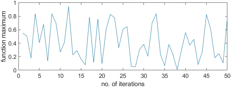
Plotting Results Of Study One
figure(2)
subplot(2,1,1)
hold on
surf(x,y,-f)
xlabel('x values')
ylabel('y values')
shading interp
plot3(xopt,yopt,-fopt,'marker','o','MarkerSize',5,'MarkerFaceColor','r')
title('without boundary condition')
subplot(2,1,2)
% to plot f maximum vs number of iterations
plot(-fopt)
xlabel('no. of iterations')
ylabel('function maximum')
study_time1 = toc;
‘Subplot’ command is used to create subplots.
‘surf’ and ‘plot3’ to plot the surface and optimal points.
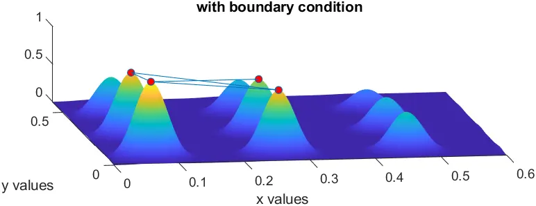
Study Two : GA With Boundary Condition
tic
for i = 1:num_cases
[inputs, fopt(i)] = ga(@stalagmite,2,[],[],[],[],[0;0],[0.6;0.6]);
xopt(i) = inputs(1);
yopt(i) = inputs(2);
end
Runs the genetic algorithm with boundary conditions [0, 0] to [0.6, 0.6].
Plotting Results Of Study Two
figure(3)
subplot(2,1,1)
hold on
surf(x,y,-f)
xlabel('x values')
ylabel('y values')
shading interp
plot3(xopt,yopt,-fopt,'marker','o','MarkerSize',5,'MarkerFaceColor','r')
title('with boundary condition')
subplot(2,1,2)
% to plot f maximum vs number of iterations
plot(-fopt)
xlabel('no. of iterations')
ylabel('function maximum')
study_time2 = toc;
Similar plotting steps as in study one.
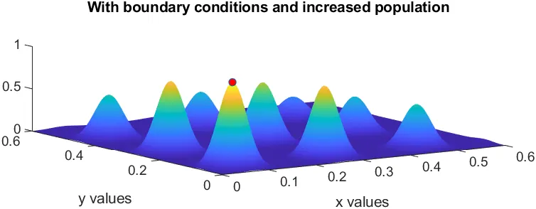
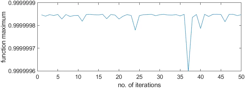
Study Three : GA With Boundary Conditions And Increased Population
tic
options = optimoptions('ga');
options = optimoptions(options,'PopulationSize',300);
for i = 1:num_cases
[inputs, fopt(i)] = ga(@stalagmite,2,[],[],[],[],[0;0],[0.6;0.6],[],[],options);
xopt(i) = inputs(1);
yopt(i) = inputs(2);
end
‘optimoptions’ is used to set a custom population size for the genetic algorithm.
Sets the population size of the genetic algorithm to 300.
Plotting Results Of Study Three
figure(4)
subplot(2,1,1)
hold on
surf(x,y,-f)
xlabel('x values')
ylabel('y values')
shading interp
plot3(xopt,yopt,-fopt,'marker','o','MarkerSize',5,'MarkerFaceColor','r')
title('With boundary conditions and increased population')
subplot(2,1,2)
% to plot f maximum vs number of iterations
plot(-fopt)
xlabel('no. of iterations')
ylabel('function maximum')
study_time3 = toc;
Similar plotting steps as in the previous studies.
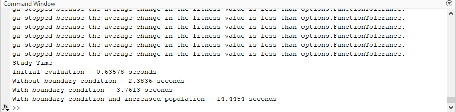
Displaying Study Times
% Display study times
disp('Study Time')
disp(['Initial evaluation = ',num2str(study_time),' seconds'])
disp(['Without boundary condition = ',num2str(study_time1),' seconds'])
disp(['With boundary condition = ',num2str(study_time2),' seconds'])
disp(['With boundary condition and increased population = ',num2str(study_time3),' seconds'])
Displays the time taken for each study.
MAIN PROGRAM
clear all
close all
clc
% Defining our search space
x = linspace(0,0.6,150);
y = linspace(0,0.6,150);
num_cases = 50;
% Creating a 2D mesh
[xx, yy] = meshgrid(x, y);
% Evaluating stalagmite function
tic
for i = 1:length(xx)
for j = 1:length(yy)
input_vector(1) = xx(i,j);
input_vector(2) = yy(i,j);
f(i,j) = stalagmite(input_vector);
end
end
figure(1)
surfc(xx,yy,-f);
xlabel('x value')
ylabel('y value')
shading interp
study_time = toc;
% Study one without boundry condition
tic
for i = 1:num_cases
[inputs, fopt(i)] = ga(@stalagmite,2);
xopt(i) = inputs(1);
yopt(i) = inputs(2);
end
figure(2)
subplot(2,1,1)
hold on
surf(x,y,-f)
xlabel('x values')
ylabel('y values')
shading interp
plot3(xopt,yopt,-fopt,'marker','o','MarkerSize',5,'MarkerFaceColor','r')
title('without boundary condition')
subplot(2,1,2)
% to plot f maximum vs number of iterations
plot(-fopt)
xlabel('no. of iterations')
ylabel('function maximum')
study_time1 = toc;
% Study two with boundary condition
tic
for i = 1:num_cases
[inputs, fopt(i)] = ga(@stalagmite,2,[],[],[],[],[0;0],[0.6;0.6]);
xopt(i) = inputs(1);
yopt(i) = inputs(2);
end
figure(3)
subplot(2,1,1)
hold on
surf(x,y,-f)
xlabel('x values')
ylabel('y values')
shading interp
plot3(xopt,yopt,-fopt,'marker','o','MarkerSize',5,'MarkerFaceColor','r')
title('with boundary condition')
subplot(2,1,2)
% to plot f maximum vs number of iterations
plot(-fopt)
xlabel('no. of iterations')
ylabel('function maximum')
study_time2 = toc;
% Study three with boundary condition and increased population
tic
options = optimoptions('ga');
options = optimoptions(options,'PopulationSize',300);
for i = 1:num_cases
[inputs, fopt(i)] = ga(@stalagmite,2,[],[],[],[],[0;0],[0.6;0.6],[],[],options);
xopt(i) = inputs(1);
yopt(i) = inputs(2);
end
figure(4)
subplot(2,1,1)
hold on
surf(x,y,-f)
xlabel('x values')
ylabel('y values')
shading interp
plot3(xopt,yopt,-fopt,'marker','o','MarkerSize',5,'MarkerFaceColor','r')
title('With boundary conditions and increased population')
subplot(2,1,2)
% to plot f maximum vs number of iterations
plot(-fopt)
xlabel('no. of iterations')
ylabel('function maximum')
study_time3 = toc;
% Display study times
disp('Study Time')
disp(['Initial evaluation = ',num2str(study_time),' seconds'])
disp(['Without boundary condition = ',num2str(study_time1),' seconds'])
disp(['With boundary condition = ',num2str(study_time2),' seconds'])
disp(['With boundary condition and increased population = ',num2str(study_time3),' seconds'])
STALAGMITE FUNCTION PROGRAM
function[f] = stalagmite(input_vector)
% f(x,y) = f1x*f1y*f2x*f2y
x = input_vector(1);
y = input_vector(2);
f1_x = (sin((5.1*pi).*x+0.5)).^6;
f1_y = (sin((5.1*pi).*y+0.5)).^6;
f2_x = exp((-4*log(2)).*(((x-0.0667).^2)/0.64));
f2_y = exp((-4*log(2)).*(((y-0.0667).^2)/0.64));
fxy = f1_x*f1_y*f2_x*f2_y;
f = -fxy;
end
OUTPUT
Initial Evaluation
Study One : GA Without Boundary Conditions
Study Two : GA With Boundary Condition
Study Three : GA With Boundary Conditions And Increased Population
Record Of Study Times
CONCLUSION
This code evaluates the performance of a genetic algorithm on the stalagmite function under different conditions and visualizes the results.