Week 5 - Genetic Algorithm

Problem Statement:

• Understand and explain the GA Concept
• Code in MATLAB to optimize the stalagmite function and find the global maxima of the given function along with the three studies showcased in the lecture.

Literature - Genetic Algorithm:

A genetic algorithm is a search heuristic inspired by the process of natural selection and genetics. It is used to find approximate solutions to optimization and search problems. The main idea is to evolve a population of candidate solutions (individuals) over multiple generations to find the best solution (fittest individual).

The GA starts with a population of random individuals (possible solutions) and evaluates their fitness using a predefined fitness function. Then, based on their fitness, individuals are selected to undergo genetic operations like crossover (combining parts of two individuals) and mutation (changing some parts of an individual). This process mimics the natural selection process, where better-fit individuals have a higher chance of survival and passing their genes to the next generation.

A genetic algorithm comprises five key phases: Initial population, Fitness function, Selection, Crossover, and Mutation.

The process kicks off with the Initial Population phase, where a group of individuals, termed a Population, is established. Each individual is defined by a set of parameters called Genes, which are combined into a Chromosome (solution).

The Fitness Function phase determines how fit each individual is by comparing them to one another. It assigns a fitness score to each individual, guiding their selection for reproduction. In optimizing genetic algorithms (GAs), the fitness function is crucial for evaluating the stalagmite function to locate its minima, typically with inputs (x, y).

Selection involves picking the fittest individuals to pass their genes to the next generation. This phase selects two pairs of individuals based on their fitness scores, with higher fitness scores increasing the chance of selection for reproduction.

Crossover is the process of creating offspring by merging genes from two parent solutions. A crossover point within the genes is randomly chosen for each pair of parents, and genes are exchanged until reaching the crossover point, resulting in new offspring added to the population.

Mutation maintains genetic diversity in the population by introducing changes from one generation to the next. This diversity prevents premature convergence and the trapping of solutions in local minima.

Advantages of genetic algorithms include their independence from derivative information, strong parallel capabilities, suitability for optimizing both continuous and discrete functions, handling of multi-objective problems, generation of multiple good solutions, effectiveness in large search spaces with numerous parameters, and consistent delivery of good results over time.

However, GAs have limitations, such as the risk of not converging to the optimal solution if not implemented correctly, and they are not ideal for simple problems with known derivative values.

Code Solution to our GA Problem - Entire with 3 Studies:

%% Creating the search space to be optimized
%one dimensional

clear all 
close all
clc

n=150;
x = linspace(0,0.6,150);
y = linspace(0,0.6,150);

%creating two dimensional grid
[xx, yy] = meshgrid(x,y);
tic

%% Case 0 
%evaluating the stalagmite function

for i = 1:length(xx)
    for j = 1:length(yy)
        input_vector(1)= xx(i,j);
        input_vector(2)= yy(i,j);
        f(i,j) = stalagmite(input_vector);
    end
end

figure(1)
surfc(xx, yy, f)
shading interp
xlabel('x value');
ylabel('y value');

study_time=toc;

%% Study 1 -  Unbounded Input Range 

%case 1 (unbounded inputs)
tic
for i = 1:n
    [inputs,fopt(i)]= ga(@stalagmite, 2);
    xopt(i)=inputs(1);
    yopt(i)=inputs(2);
end

figure(2)
subplot(2,1,1)
hold on
surfc (x,y,-f)
shading interp
plot3(xopt,yopt,-fopt,'marker','o','markersize',5,'markerfacecolor','r')
title('unbounded inputs')
subplot(2,1,2)
plot(-fopt)
xlabel('no. of iterations');
ylabel('function max');

study_time1=toc;

%% Case 2 Bounded Inputs
tic
for i = 1:n
    [inputs,fopt(i)]= ga(@stalagmite, 2,[],[],[],[],[0;0],[0.6;0.6]);
    xopt(i)=inputs(1);
    yopt(i)=inputs(2);
end

figure(3)
subplot(2,1,1)
hold on
surfc (x,y,-f)
shading interp
plot3(xopt,yopt,-fopt,'marker','o','markersize',5,'markerfacecolor','r')
title('bounded inputs')
subplot(2,1,2)
plot(-fopt)
xlabel('no. of iterations');
ylabel('function max');

study_time2=toc;

%% Case 3 - bounded inputs with increased population

tic
options=optimoptions('ga');
options=optimoptions(options,'PopulationSize',500);

for i = 1:n
    [inputs,fopt(i)]= ga(@stalagmite,2,[],[],[],[],[0;0],[1;1],[],[],options);
    xopt(i)=inputs(1);
    yopt(i)=inputs(2);
end

figure(4)
subplot(2,1,1)
hold on
surfc (x,y,-f)
shading interp
plot3(xopt,yopt,-fopt,'marker','o','markersize',5,'markerfacecolor','r')
title('bounded inputs with increases population')
subplot(2,1,2)
plot(-fopt)
xlabel('no. of iterations');
ylabel('function max');

study_time3=toc;

Results and Explanation:

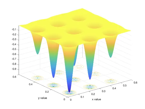
Initially we'll take a look at the stalagmite function's plot which we have to optimise. Then we start with the specific case studies

Plot for the Stalgmite Function:

Case Study 1: Statistical behavior with unbounded inputs

- Process:

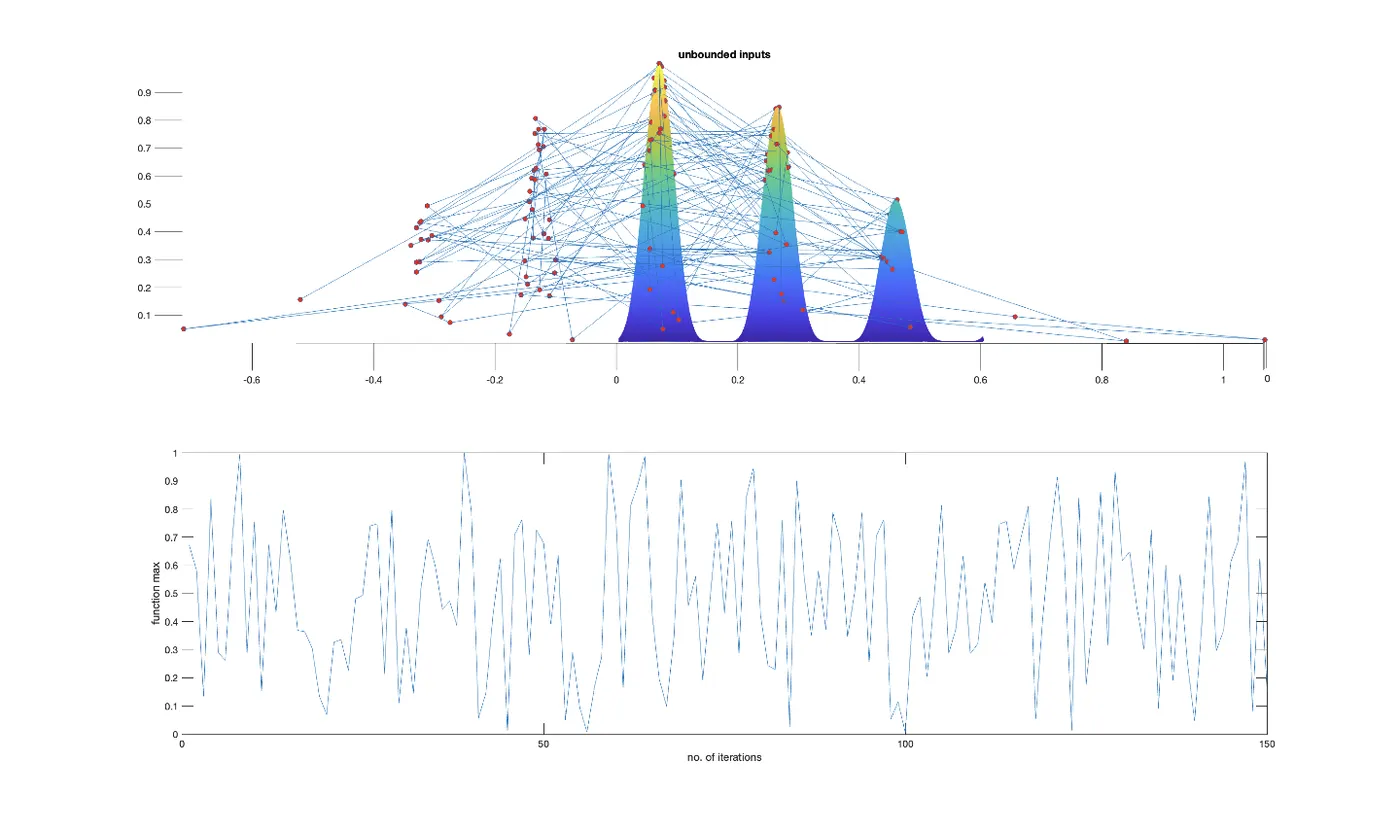
- The GA solver is called in a loop for 150 iterations without specifying any constraints on the search space.

- The results are plotted using surf and plot3 commands to visualize the 3D representation of the stalagmite function with optimization results and function value trends over iterations.

- Findings:

- The GA solver is iterated 150 times without any upper or lower limits on the input variables.

- The solver returns minimum function values (fopt) and the corresponding coordinates (xopt, yopt) for each iteration.

- The maximum value of the function ranges between 0.1 to 1 due to random sampling, indicating that further optimization is needed.

- Plots:

Case Study 2: Bounded inputs

- Process:

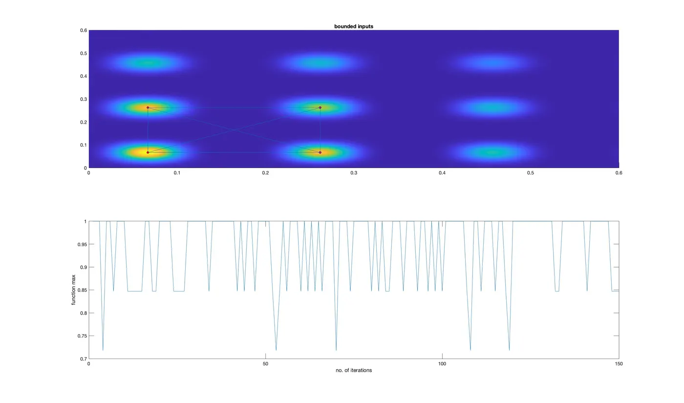
- The GA solver is called with specified upper and lower bounds for the input variables.

- Four null vectors are passed as placeholders for linear inequalities since no linear inequalities are involved in the stalagmite function.

- The results are plotted to show the optimized function value trends and the 3D representation of the stalagmite function with optimization results.

- Findings:

- The bounded inputs provide clearer results compared to unbounded inputs, with the maximum function value ranging between 0.7 to 1.

- The optimization is more focused within the specified bounds, leading to improved accuracy in finding the global minimum.

- The GA solver is run with bounds [0, 0.6] for both x and y variables.

-Plots

Case Study 3: Bounded inputs with increased population size

- Process:

- The GA solver is called with increased population size and bounded inputs.

- The optimoptions command is used to create optimization options and specify the population size.

- The results are plotted to visualize the optimized function value trends and the 3D representation of the stalagmite function with optimization results.

- Findings:

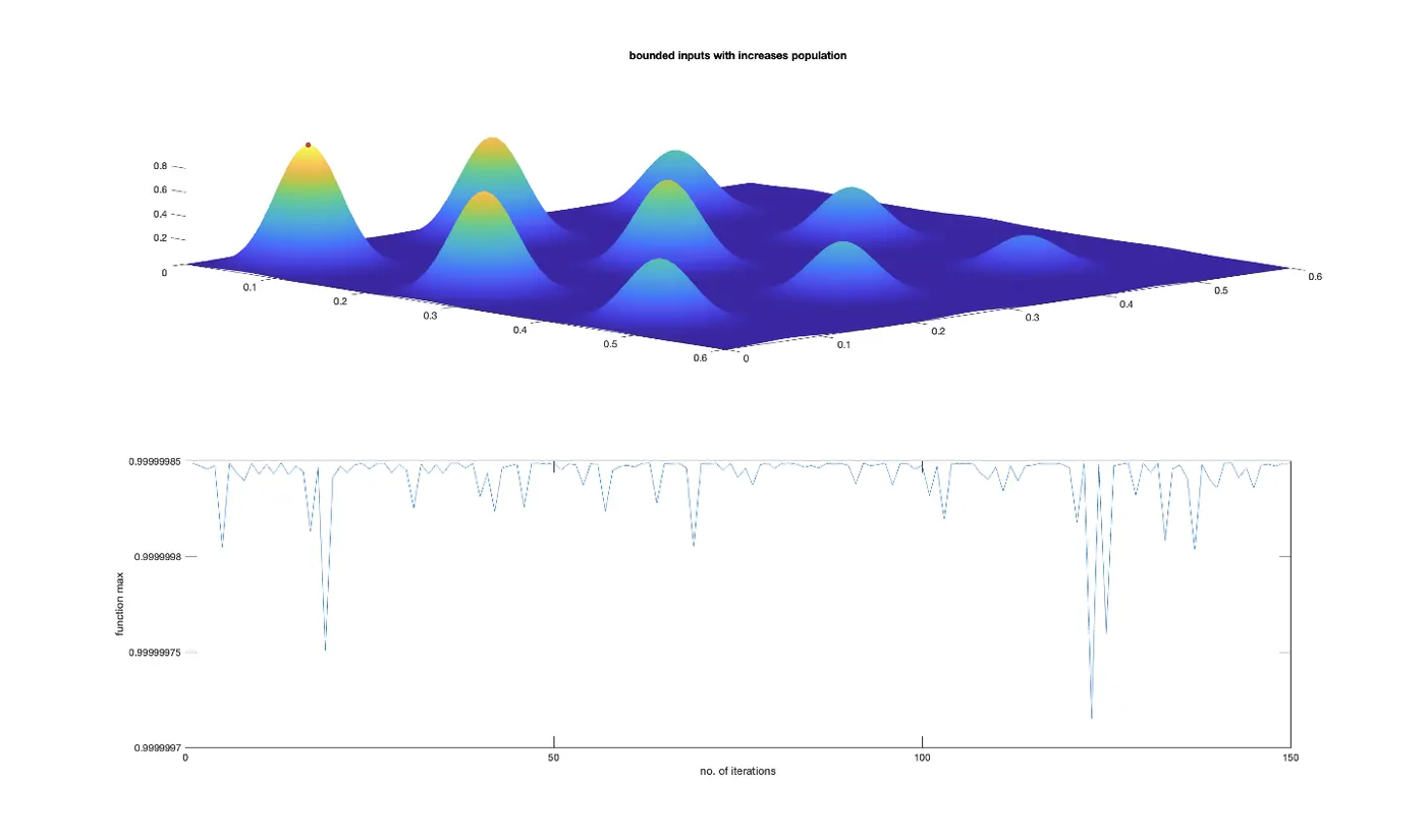
- The maximum function value obtained ranges between 0.99999980 to 0.99999985, indicating significant improvement over previous cases.

- With the increased population size, the GA explores the solution space more thoroughly, resulting in the most accurate results.

- The GA solver is run with a population size of 500 individuals per generation.

- Plots