Week 4.1 - Solving second order ODEs

Problem Statement:

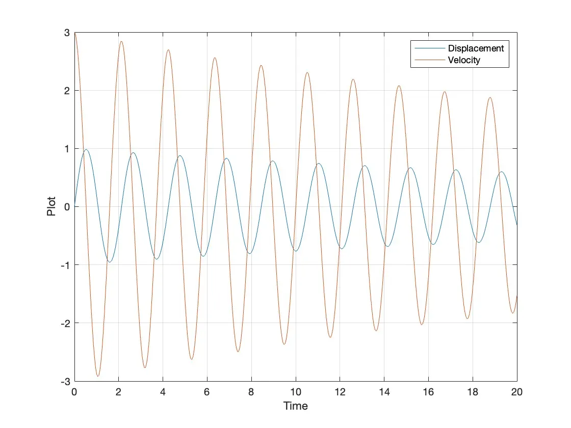
We use the ode solver to create a transient simulation of a simple pendulum.

Solution Code:

% Inputs
damping_coefficient = 0.05;
gravitational_acceleration = 9.81;
pendulum_length = 1;
pendulum_mass = 1;

initial_theta = [0; 3]; % Initial conditions for displacement and velocity
time_span = linspace(0, 20, 400); % Time span points

% Solving ODE
[t, results] = ode45(@(t, theta) ode_pendulum(t, theta, damping_coefficient, gravitational_acceleration, pendulum_length, pendulum_mass), time_span, initial_theta);

% Plotting displacement and velocity
figure(1)
plot(t, results(:, 1))
hold on
grid on
plot(t, results(:, 2))
ylabel('Plot')
xlabel('Time')
legend('Displacement', 'Velocity')

% Animation
figure(2)
for i = 1:length(results(:, 1))
    theta_1 = results(i, 1);
  
    % Initial coordinates
    x0 = 0;
    y0 = 0;

    x1 = pendulum_length * sin(theta_1);
    y1 = -pendulum_length * cos(theta_1);

    % Plot
    plot([-0.5 0.5], [0, 0], 'color', 'g') % Pivot point
    line([x0 x1], [y0 y1], 'color', 'r') % Pendulum rod
    hold on
    plot(x1, y1, 'marker', 'o', 'markersize', 25, 'MarkerFaceColor', 'b') % Pendulum bob
    grid on
    axis([-1.5 1.5 -1.5 1])
    hold off
    pause(0.0001)
    M(i) = getframe(gcf);
end

% Create animation file
videofile = VideoWriter('Damped_Pendulum_Animation.avi', 'Motion JPEG AVI');
open(videofile)
writeVideo(videofile, M)
close(videofile)


function [dtheta_dt] = ode_pendulum(t, theta, b, g, L, m)
% ODE function representing the equation of motion for a damped pendulum
% Inputs:
%   t: Time
%   theta: Vector containing angular displacement and velocity
%   b: Damping coefficient
%   g: Gravitational acceleration
%   L: Length of the pendulum
%   m: Mass of the pendulum bob
% Output:
%   dtheta_dt: Derivative of theta with respect to time

theta1 = theta(1);
theta2 = theta(2);

dtheta1_dt = theta2;
dtheta2_dt = -(b/m)*theta2 - (g/L)*sin(theta1);

dtheta_dt = [dtheta1_dt; dtheta2_dt];
end

Stepwise Explanation of the Code:

1. Function Definition (ode _ pendulum):

This function defines the ordinary differential equation (ODE) representing the motion of a damped pendulum. It takes as input the current time ('t'), the vector of angular displacement and velocity ('theta'), and parameters such as the damping coefficient ('b'), gravitational acceleration ('g'), pendulum length ('L'), and pendulum mass ('m'). It returns the derivative of the angular displacement with respect to time.

2. Main Program:

- Initialization:

- Sets up parameters such as damping coefficient, gravitational acceleration, pendulum length, and pendulum mass.

- Specifies the initial conditions for the pendulum's displacement and velocity.

- Defines the time span for simulation.

- ODE Solver ('ode45'): Solves the ODE using the provided function ('ode_pendulum') and initial conditions over the specified time span.

- Plotting:

- Plots the displacement and velocity of the pendulum over time.

- Animation:

- Iterates through each time step and calculates the position of the pendulum bob.

- Plots the pendulum rod and bob, updating the plot for each time step to create an animation.

- Captures each frame of the animation.

- Video Creation:

- Writes the captured frames into a video file to create the animation.

Errors Faced while Programming:

1. Index out of Bounds Error: This error occurred when trying to plot start and end points in the animation. It was caused by an empty array ('start_points' or 'end_points') being accessed without checking if it was empty first.

How Errors were Overcome:

1. Index out of Bounds Error:

- To resolve this error, a check was added to ensure that the array ('start_points' or 'end_points') was not empty before plotting its contents. This prevented the code from attempting to access non-existent array elements.

Output and Results:

Youtube Link