Week 5 - Genetic Algorithm

Week 5 - Genetic Algorithm:

Aim:

• To Write a code in MATLAB to optimise the stalagmite function and find the global maxima of the function.
• To Clearly expalin the concept of genetic algorithm in your own words and also explain the syntax for ga in MATLAB in your report.
• To Make sure that your code gives the same output, even if it is made to run several times.
• To Plot graphs for all 3 studies and for F maximum vs no. of iterations. Title and axes labels are a must, legends could be shown if necessary.

Genetic Algorithm Introduction:

• A genetic algorithm (GA) is a computational optimization technique that uses the principles of natural selection and genetics to solve complex problems.
• GAs are based on Charles Darwin's theory of natural selection and were developed in the 1960s and 1970s by John Holland and his collaborators
• GAs mimic the process of natural selection to evolve a population of potential solutions to an optimization problem.
• This is achieved through a process of selection, crossover, and mutation, which iteratively improves the quality of the solutions over multiple generations.

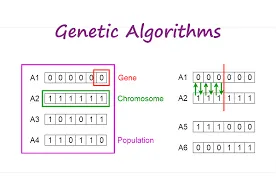
• GAs are made up of three different operators: selection, crossover, and mutation. The GA solution is encoded in a binary string known as chromosome. The elements of a chromosome are referred to as genes.
• GAs are used in science and engineering as adaptive algorithms for solving practical problems and as computational models of natural evolutionary systems. They are also used to solve optimization problems in machine learning.

Challenge Solution:

Stalagmite relation with mathematical model:

• In a mathematical context, a stalagmite could be represented as a geometric shape or a function that describes its form. Stalagmites are formations that grow upward from the floor of a cave due to the deposition of mineral-rich water.
• The mathematical modeling of stalagmite growth might involve various factors, such as the rate of mineral deposition, environmental conditions, and time.

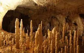
Here is a simple conceptual model:

• Let h(t) represent the height of the stalagmite at time t. The rate of growth could be proportional to the current height, and it might be affected by other environmental factors. You could formulate a differential equation like:

• dh/dt =k⋅h(t)+f(t)
• where:
• k is a growth constant.
• f(t) represents additional factors influencing the growth.

Stalagmite with Generic algorithm:

• To optimize or model stalagmite growth using a generic algorithm, you would typically employ an optimization algorithm that is inspired by the principles of natural selection and genetics.
• One commonly used generic algorithm is the Genetic Algorithm (GA).

optimise the stalagmite function and find the global maxima of the function:

Study 1:Statistical behavior without bounds:

Now come to our study,For that we need to do given below steps,

• Define the Function: Clearly define the mathematical function you want to optimize. For example, if your function is denoted as f(x), write it down explicitly.
• Find Derivatives: Calculate the first and second derivatives of your function with respect to the variable you are optimizing. These derivatives help identify critical points where the function reaches a maximum or minimum.
• Solve for Critical Points: Set the first derivative equal to zero and solve for the variable to find critical points. Also, check for points where the derivative is undefined.
• Use the Second Derivative Test: Evaluate the second derivative at each critical point. If the second derivative is positive, the critical point corresponds to a local minimum; if negative, it corresponds to a local maximum.
• Check Endpoints: If your function is defined over a specific interval, check the values of the function at the endpoints of that interval.
• Evaluate Function at Critical Points and Endpoints: Plug the critical points and endpoint values into the original function to find the corresponding function values.
• Compare Results: Compare the function values obtained from steps 4 and 6 to identify the global maximum.

First we need to create the function called stalagmite Ga,

Statistical behavior without bounds Code line by line explaination:

• x = linspace(0,0.6,150); - linspace command is used for providing intervals with a given value, where the value for x and y is given and these are the input arrays of x and y.
• y = linspace(0,0.6,150) - linspace command is used for providing intervals with a given value, where the value for x and y is given and these are the input arrays of x and y.
• num_cases = 50; - num cases is 50 called the genetic algorithm to run for 50 times
• [xx,yy] = meshgrid(x,y); - the command is used to mesh the 2D or 3D plot, where x and y are the axis the plots to meshed.
• for i = 1:length(xx) - for loop is created for repeating the set of values with respective to x-axis.
• for j = 1:length(yy) - for loop is created for repeating the set of values with respective to x-axis.
• input_vector(1) = xx(i,j); - for each value of x basically an array is created called input_vector.
• input_vector(2) = yy(i,j); - for each value of y basically an array is created called input_vector.
• f(i,j) = stalagmite(input_vector); - Where stalagmite is a function. The stalagmite takes the input_vector and calculates the f.
• end - The command must be used when for loop is called.
• tic - the command is used to calculate the operation time performed.
• [inputs, fopt(i)] = ga(@stalagmite, 2); where the study for statistical behaviour is started with inputs and fopt(i) are the variables for the given input. stalagmite is a function a code is written seperately and called for the operation. 2 is the no of variables as inputs.
• xopt(i) = inputs(1); - the x value for the input is wriiten with the variable called xopt.# yopt(i) = inputs(2); - the y value for the input is wriiten with the variable called yopt.
• end - forloop is called so end must be used
• study_time1 = toc -the command is used to calculate the operation time performed for study1.
• subplot(2,1,1) - The subplot command is used for creating multiple plot with a plot. The 2,1 is the x and y axis with respective to first column.
• hold on - the command is used for adding new elements for showing the graph.
• surfc(x,y,-f) - surfc command is used for creating the surface for the function.
• shading interp - the command is used to plot the 3D graph where the grid on the 3D will be as smooth shading.
• plot3(xopt,yopt,-fopt,'marker','o','markersize',5,'markerfacecolor','r') the command is used for plotting the x,y,z axis in the graph. The marker and markersize command are used to created the size and shape of the maxima.
• title('unbounded inputs') - the command used to represent the graph name.
• subplot(2,1,2) - The subplot command is used for creating multiple plot with a plot. The 2,1 is the x and y axis with respective to second column.
• plot(-fopt) - (-fopt) is given to plot the graph in maxima.
• xlabel('iterations') - xlabel is the command used for creating x-axis name.
• ylabel('function maximum') - ylabel is the command used for creating y-axis name.

Output:

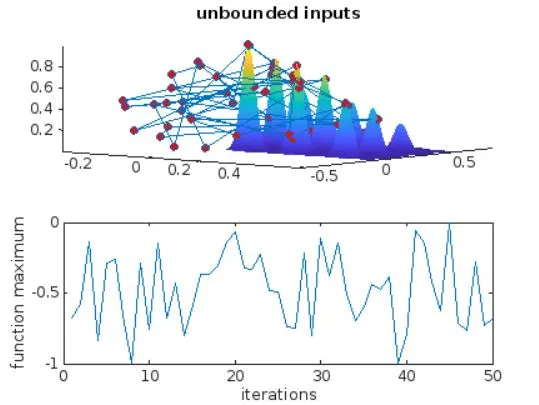
• study_time1 = 4.22 secs is the time taken to execute study1.
• The value for x = 0.0666
• The value for y = 0.0656
• The value for z = 0.996 this is the minimum obtained from x and y.

Study 2:statistical behaviours with upper and lower bounds:

CODE for statistical behaviours with upper and lower bounds:

Code explaination:

• for i = 1:num_cases: This line starts a loop that will run num_cases times, where num_cases is the number of cases you want to study.
• [inputs, fopt(i)] = ga(@stalagmite,2,[],[],[],[],[0;0],[0.6;0.6]);: This line performs a genetic algorithm (GA) optimization using the ga function.
• It optimizes the stalagmite function, which takes 2 input variables. The optimization is performed within the specified bounds [0;0] and [0.6;0.6].
• The optimized inputs are stored in the inputs variable, and the corresponding function value is stored in fopt(i) for the current iteration i.
• xopt(i) = inputs(1); and yopt(i) = inputs(2);: These lines extract the optimized values of x and y from the inputs variable and store them in the arrays xopt and yopt for the current iteration i.
• end: This marks the end of the loop. The loop runs for num_cases iterations, optimizing the stalagmite function with the genetic algorithm each time.
• study_time2 = toc;: This line records the time taken for the entire loop to run using the toc function.
• figure(2): This creates a new figure with the number 2.
• subplot(2,1,1): This creates a subplot grid with 2 rows and 1 column, and it selects the first subplot for the following plotting.
• surf(x,y,-f): This plots a 3D surface plot using the x, y, and -f (negation of the stalagmite function) values.
• shading interp: This command interpolates the color between the data points in the surface plot.
• hold on: This command allows for additional plot elements to be added to the existing plot.
• plot3(xopt, yopt, -fopt,'marker','o','markersize',5,'markerfacecolor','r'): This line adds a 3D plot of the optimized points (xopt, yopt, -fopt) to the existing surface plot. The points are marked with red circles.
• title('bounded inputs'): This sets the title of the subplot to 'bounded inputs'.
• subplot(2,1,2): This selects the second subplot in the 2-row, 1-column subplot grid.
• plot(-fopt): This line plots the negation of the function maximum values over iterations.
• xlabel('iterations') and ylabel('function maximum'): These lines label the x-axis as 'iterations' and the y-axis as 'function maximum' for the second subplot.

Output for statistical behaviours with upper and lower bounds:

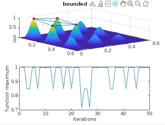
• Study_time2 = 5.25 secs is the time taken to execute Study2
• The value for x = 0.0666
• The value for y = 0.0686
• The value for z = 1 this is the minimum obtained from x and y.

Study 3:Increasing ga iterations:

Code for Study 3:Increasing ga iterations:

Code line by line explaination:

• options = optimoptions('ga');: This line creates a structure named options using the optimoptions function for the genetic algorithm. By default, it uses the settings for the genetic algorithm.
• options = optimoptions(options, 'populationsize', 500);: This line updates the options structure to set the population size for the genetic algorithm to 500. This increases the number of individuals in each generation.
• tic: This command starts a stopwatch timer.
• for i = 1:num_cases: This line starts a loop that will run num_cases times.
• [inputs, fopt(i)] = ga(@stalagmite, 2, [], [], [], [], [0;0], [0.1;0.1], [], [], options);: This line uses the genetic algorithm (ga) to optimize the stalagmite function with the following settings:
• @stalagmite: The function to be optimized.
• 2: The number of variables in the optimization problem.
• []: No linear inequality constraints.
• []: No linear equality constraints.
• []: No nonlinear inequality constraints.
• []: No nonlinear equality constraints.
• [0;0]: Lower bounds for the optimization variables.
• [0.1;0.1]: Upper bounds for the optimization variables.
• []: No initial guess.
• []: No options structure is passed; the default options are used.
• xopt(i) = inputs(1); and yopt(i) = inputs(2);: These lines store the optimized values of x and y for the current iteration i.
• end: This marks the end of the loop. The loop runs for num_cases iterations.
• study_time3 = toc;: This line records the time taken for the entire loop to run using the toc function.
• figure(3): This creates a new figure with the number 3.
• subplot(2,1,1): This selects the first subplot in a 2-row, 1-column subplot grid for the following plotting.
• hold on: This allows for additional plot elements to be added to the existing plot.
• surf(x, y, -f): This plots a 3D surface plot using the x, y, and -f (negation of the stalagmite function) values.
• shading interp: This command interpolates the color between the data points in the surface plot.
• plot3(xopt, yopt, -fopt, 'marker', 'o', 'markersize', 5, 'markerfacecolor', 'r'): This line adds a 3D plot of the optimized points (xopt, yopt, -fopt) to the existing surface plot. The points are marked with red circles.
• title('bounded inputs with increasing ga'): This sets the title of the subplot to 'bounded inputs with increasing ga'.
• subplot(2,1,2): This selects the second subplot in the 2-row, 1-column subplot grid.
• plot(-fopt): This line plots the negation of the function maximum values over iterations.
• xlabel('iterations') and ylabel('function maximum'): These lines label the x-axis as 'iterations' and the y-axis as 'function maximum' for the second subplot.

Output for Study 3:Increasing ga iterations:

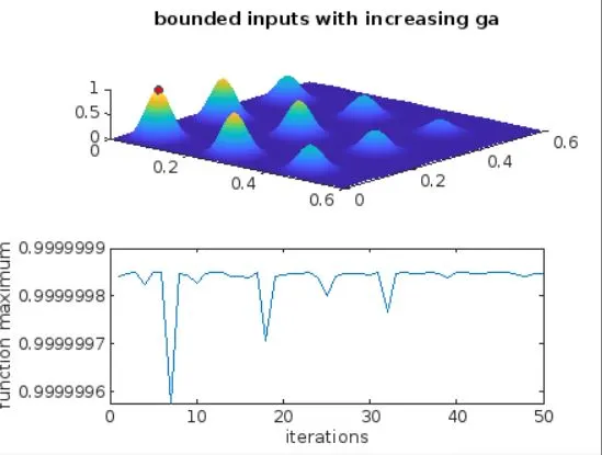
• study_time3 = 36.42 secs is the time taken to execute study3.
• The value for x = 0.0683
• The value for y = 0.0643
• The value for z = 0.9934 this is the minimum obtained from x and y.

Theory about Genetic Algorithm:

• Genetic Algorithms (GAs) are optimization and search heuristics inspired by the process of natural selection.
• They are part of the broader class of evolutionary algorithms and have been successfully applied to a wide range of optimization problems.
• The underlying theory and principles of genetic algorithms include the following key concepts:
• Inspiration from Natural Selection:
  
  • Genetic Algorithms are based on the idea of mimicking the process of natural selection and evolution.
  • In nature, species evolve over time through the mechanism of survival of the fittest. Similarly, GAs evolve a population of potential solutions to a problem, with the fittest individuals having a higher chance of being selected for reproduction.
• Population Representation:
  
  • In GAs, a population of candidate solutions is maintained, with each solution representing a potential solution to the problem at hand.
  • Solutions are often encoded as strings of values, known as chromosomes.
• Chromosomes and Genes:
  
  • Chromosomes are structures that represent individuals in the population.
  • They are composed of genes, which are the specific parameters or variables that define a solution.
  • The combination of genes forms a potential solution.
• Selection:
  
  • The selection process in GAs is analogous to natural selection.
  • Individuals with better fitness, determined by how well they solve the problem at hand, have a higher probability of being selected to "reproduce."
• Crossover (Recombination):
  
  • Crossover is the process of combining genetic information from two parent solutions to create new offspring.
  • This mimics the idea of genetic recombination in biological reproduction.
• Mutation:
  
  • Mutation introduces small random changes to the genetic information, helping to maintain genetic diversity in the population.
  • It ensures that new solutions are explored, even if they are not directly inherited from parents.
• Fitness Function:
  
  • The fitness function evaluates how well a solution performs the task at hand.
  • It quantifies the quality of a solution, and individuals with higher fitness values are favored in the selection process.
• Generational Evolution:
  
  • GAs operate in generations. In each generation, the population undergoes selection, crossover, and mutation, producing a new generation of individuals.
  • Over successive generations, the population tends to improve as better solutions are discovered.
• Termination Criteria:
  
  • The algorithm terminates when a certain condition is met, such as finding a satisfactory solution, reaching a maximum number of generations, or achieving a specific level of fitness.
• Application to Optimization Problems:
  
  • GAs are particularly well-suited for optimization problems, where the goal is to find the best solution among a large search space.
  • They have been successfully applied in various domains, including engineering, finance, scheduling, and machine learning.
• Adaptation and Exploration:
  • GAs strike a balance between exploitation (refining current solutions) and exploration (searching for new solutions). This balance allows them to navigate complex solution spaces effectively.

Conclusion:

• This project used Genetic Algorithms to find the best solutions for a tricky math problem called the stalagmite function.
• The studies showed that Genetic Algorithms can handle a wide range of solutions when there are no specific limits.
• When we set limits for the solutions, Genetic Algorithms still worked well, showing they're good for problems with constraints.
• By running the Genetic Algorithm more times, the project found that it could get even better results over time.
• The complex math used in the stalagmite function made it a tough challenge, but Genetic Algorithms showed they are flexible and effective for solving such tricky problems.