Week 5 - Genetic Algorithm

The genetic Algorithm works like Campus Recruitment or the job interveiws.

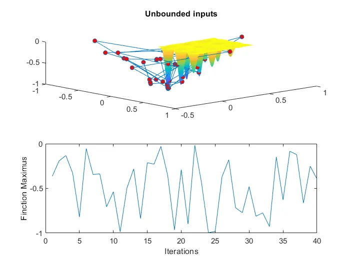
Unbounded inputs:-The minimum criteria, clear the subjects within academic year. Here,the no.of people will be more and time taken to select the candidates will be less.

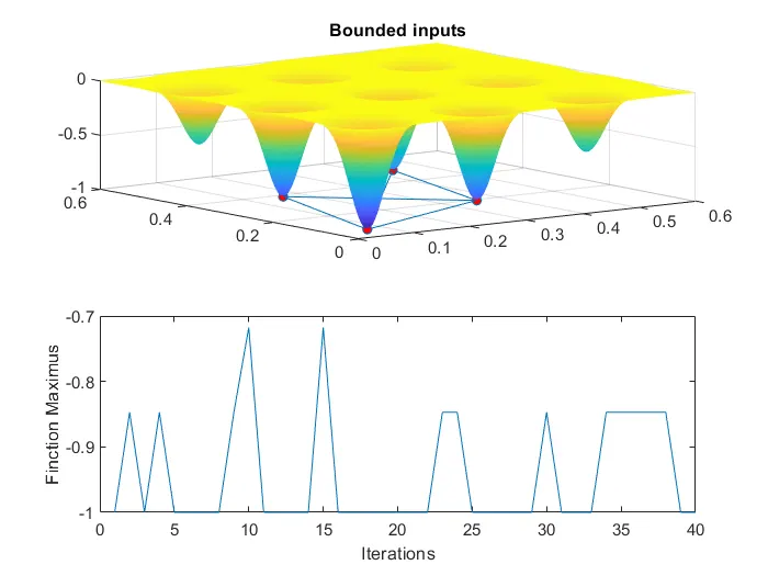
Bounded inputs:- The second criteria is to have nice CGPA,Aptitude and others.Here,the no.of people will be moderate and time taken to select the candidates will be moderate.

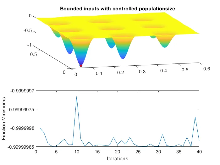
Controlled Population:- Amongs the large population of the merit candidates finding the skilled person will be diffcult and it takes more time.

Syntax of GA(ga):-

x=ga(function,no.of variables)

x=ga(function,no.of variables,A,b,Aeq,beq,lb=lower bounds,ub=upper bounds) (imp:- set A=[], b= [], Aeq=[], beq=[], if no linear inequalities exist.)

Stalagmite Function:-

function [f] = stalagmite(input_vector)
    x = input_vector(1);
    y = input_vector(2);
    f1_x = (sin(5.1 * pi * x + 0.5))^6;
    f2_x = exp(-4 * log(2) * ((x - 0.0667)^2) / 0.64);
    f1_y = (sin(5.1 * pi* y + 0.5))^6;
    f2_y = exp(-4 * log(2) * ((y - 0.0667)^2) / 0.64);
    f = -f1_x*f2_x*f1_y*f2_y; % '-' is for maximum
end

Main Code:-

%%
% Clear workspace, close figures, and clear command window
clear
clear
close all
clc

% Generate a grid of points for visualization
x=linspace(0,0.6,150);
y=linspace(0,0.6,150);
[xx yy]=meshgrid(x,y);

% Evaluate the stalagmite function on the grid
for i=1:length(xx)
     for j=1:length(yy)
           input_vector(1)=xx(i,j); 
           input_vector(2)=yy(i,j); 
           f(i,j)=stalagmite(input_vector); 
     end
end

% Run GA to find the optimal solution for stalagmite function
[inputs,fval] = ga(@stalagmite,2); 
x_out = inputs(1);
y_out = inputs(2);
xlabel('x-axis') 
ylabel('y-axis') 

%%
% Case 1: Unbounded inputs, a limited number of iterations
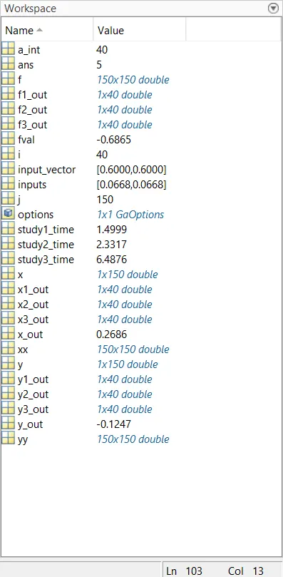
a_int = 40; %no.of iteration

tic 
for i=1:a_int
     
    [inputs,f1_out(i)] = ga(@stalagmite,2); 
    x1_out(i) = inputs(1);
    y1_out(i) = inputs(2);

end
study1_time = toc; 5 
figure(1)
subplot(2,1,1) 
hold on
surf(xx,yy,f) 
shading interp
plot3(x1_out,y1_out, f1_out,'Marker','o', 'MarkerSize',5,'MarkerFaceColor', 'r') 
title('Unbounded inputs') 
subplot(2,1,2) 
plot(f1_out)
xlabel('Iterations')
ylabel('Finction Maximus')

%%
% Case 2: Bounded inputs, a limited number of iterations
tic 
for i=1:a_int
     
    [inputs,f2_out(i)] = ga(@stalagmite,2,[],[],[],[],[0;0],[0.6;0.6])  
    x2_out(i) = inputs(1);
    y2_out(i) = inputs(2);

end
study2_time=toc;  

% Plot results for Case 2
figure(2)
subplot(2,1,1)
surf(xx,yy,f) 
hold on
shading interp
plot3(x2_out,y2_out, f2_out,'Marker','o', 'MarkerSize',5,'MarkerFaceColor', 'r')
title('Bounded inputs')
subplot(2,1,2)
plot(f2_out)
xlabel('Iterations')
ylabel('Finction Maximus')

%%
% Case 3: Bounded inputs with controlled population size
options = optimoptions('ga'); % Method to initialize stopping period for GA we used this code as we are providing a stopping period for a solver which is dependant on some other function.
options = optimoptions(options,'PopulationSize',200);

tic % used for calculating the time loop takes to complete compiling
for i=1:a_int
     
    [inputs,f3_out(i)] = ga(@stalagmite,2,[],[],[],[],[0;0],[0.6;0.6],[],[],options); % Declaration of GA with boundry conditions and stopping criteria
    x3_out(i) = inputs(1);
    y3_out(i) = inputs(2);

end
study3_time = toc % Calculates compiling time for the loop 

% Plot results for Case 3
figure(3)
subplot(2,1,1)
hold on
surf(xx,yy,f) % creates a surface for given parametrs
shading interp
plot3(x3_out,y3_out, f3_out,'Marker','o', 'MarkerSize',5,'MarkerFaceColor', 'r')
title('Bounded inputs with controlled populationsize')
subplot(2,1,2)
plot(f3_out)
xlabel('Iterations')
ylabel('Finction Minimums')

Results:-