Week 4.1 - Solving second order ODEs

ODE FUNCTIONAL CODE:-

%%
% function code
function[dtheta_dt]= ode_func(t,theta)
b = 0.05; % given values of consider this values as constant.
g = 9.81;
l = 1;
m = 1;
theta1=theta(1);
theta2=theta(2);
dtheta1_dt=theta2; %First element is angular velocity ,which is at theta(2) position
dtheta2_dt=-(b/m)*theta2-(g/l)*sin(theta1); % This will obtain after conversion of 2nd order ODE to 1st order ODE.
dtheta_dt=[dtheta1_dt; dtheta2_dt]; % allocating dtheta1_dt into row 1 and dtheta2_dt into row2 and storing in variable dtheta_dt.
end

ODE MAIN CODE:-

clear
close all
clc

%%
%
l=1;
theta_0 = [0 5];

t_span = linspace(0,20,500); % 0 to 10,500 equal point.

% this below step is for solving differential equation using ode45
% syntax for ode45[t,y] = ode45(odefun,tspan,y0), where tspan = [t0 tf], integrates the system of differential equations y′=f(t,y) from t0 to tf with initial conditions y0. Each row in the solution array y corresponds to a value returned in column vector t.
[t, results]= ode45('ode_func',t_span, theta_0);

%plotting for tracing of angular velocity and angula displacement
subplot(2,1,1)
plot(t,results(:,1));
xlabel('time t in sec');
ylabel('Angular displacement');

hold on 

subplot(2,1,2)
plot(t,results(:,2))
ylabel('Plot')
xlabel('time')
grid on
%%
% Animation
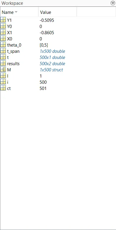
X0=0;
Y0=0;

ct=1;% counter actually represents each and every frame

% for loop starts from 1 to length of t which is 20 sec
for i=1:length(t)
    X1=l*sin(results(i,l));
    Y1=-l*cos(results(i,l));
    
    figure(2)
    plot([-1 1],[0 0],'linewidth',6,'color','g');%It goes from x=-1 to x=1 and stays at y=0.
    axis([-2 2 -2 2]);%The x-axis ranges from -2 to 2, and the y-axis also ranges from -2 to 2.syntax axis([-x x   -y y]).
    line([X0 X1],[Y0 Y1],'linewidth',2,'color','b')
    hold on,
    plot(X0,Y0,'O','markersize',5,'markerfacecolor','r');%plots a red circle (marker 'O') at the coordinates (X0,Y0) representing the fixed point.
    plot(X1,Y1,'O','markersize',30,'markerfacecolor','y');%plots a yellow circle (marker 'O') at the coordinates (X1,Y1) representing the bob of the pendulum.
    title('Damping of simple pendulum');
    legend('Support rod','length of pendulum','fixed point','bob of pendulum');
    grid on;
    hold off;
    M(ct)=getframe(gcf);%This captures the current figure as a frame in the video. The frames are stored in an array M.
    ct=ct+1;%This increments the counter ct.
end
%This plays the frames stored in M as a movie.
movie(M);
%This creates a video writer object named videofile for creating a video file. It specifies that the video will be an uncompressed AVI file.
videofile=videowriter('simple_pendulum','Uncompressed AVI');
%the video file for writing.
open(videofile);

writeVideo(videofile,M);
close(videofile);

ERROR:-

Cannot find an exact (case-sensitive) match for 'videowriter'

The closest match is: VideoWriter in M:\original matlab

installation\Polyspace\R2021a\toolbox\matlab\audiovideo\VideoWriter.m

Error in ode (line 58)

videofile=videowriter('ode.avi','Uncompressed AVI');

OUTPUT:-

https://youtu.be/8lRZ_UPRjQk

https://youtu.be/C90Bj7nqTwE