Project 2 - Rankine cycle Simulator
Main Code:-
clear
close all
clc

fprintf(' SIMULATOR OF RANKINE CYCLE \n')
fprintf('1-2 Isentropic Expansion in the Turbine\n')
fprintf('2-3 Constant Pressure Heat Rejection by the Condenser\n')
fprintf('3-2 Isentropic Compression in the Pump\n')
fprintf('4-1 Constant Pressure Heat Addition by the Boiler\n\n')
%inputs
P1 = input('Enter the Pressure at the Turbine Inlet (in bar): ');
T1 = input('Enter the Temperature at the Turbine inlet (in Degree celsius): ');
P2 = input('Enter the Pressure at the Condenser (in bar): ');
disp('RESULTS')
%getting Cp and cv values from Xsteam
%Cp and Cv assumed to not change with temperature to make problem simple
% for vapour
high_cpV= XSteam('CpV_p', P1);
low_cpV=XSteam('CpV_p', P2);
high_cvV=XSteam('CvV_p', P1);
low_cvV=XSteam('CvV_p', P2);
% for liquid
high_cpL= XSteam('CpL_p', P1);
low_cpL=XSteam('CpL_p', P2);
high_cvL=XSteam('CvL_p', P1);
low_cvL=XSteam('CvL_p', P2);
%Getting important parameters from Xsteam
%for high pressure
T1s = XSteam('Tsat_p', P1);
S1g = XSteam('sV_p', P1);
S1f = XSteam('SL_p', P1);
S1fg = S1g - S1f;
H1f = XSteam('hL_p', P1);
H1g = XSteam('hV_p', P1);
H1fg = H1g - H1f;
%for low pressure
S2g = XSteam('sV_p', P2);
S2f = XSteam('SL_p', P2);
S2fg = S2g - S2f;
T2s = XSteam('Tsat_p', P2);
H2f = XSteam('hL_p', P2);
H2g = XSteam('hV_p', P2);
H2fg = H2g - H2f;
%% State point 1
disp('At state point 1:')
fprintf('P1 is : %f Bar\n', P1)
fprintf('T1 is : %f Deg celsiusn\n', T1)
H1 = XSteam('h_pt', P1, T1);
fprintf('H1 is : %f kJ/kg\n', H1)
S1 = XSteam('s_pt', P1, T1);
fprintf('S1 is : %f kJ/kgK\n\n', S1)
%% State point 2
disp('At state point 2:')
fprintf('P2 is : %f Bar\n', P2) %P2 input already taken
S2 = S1;
fprintf('S2 is : %f kJ/kgK\n', S2)
%predicting location of point 2 in T-s
if(S2<=S2g)
 X2 = (S2 - S2f) / (S2fg); % Dryness Fraction at state point 2
else
 X2=1;
end
fprintf('X2 is :%f \n', X2)
%calculating T2 for superheat or wet or dry wherever it lies
if(X2<1)
 T2=T2s;
else
 %t2 cal by s2=s2g+low_cpV*(log(T2/T2s))
 T2=(T2s+273.15)*exp((S2-S2g)/low_cpV) ; %2 in superheated region
 T2=T2-273.15;
end
fprintf('T2 is : %f Deg celsius \n', T2)
if(X2<1)
 H2 = H2f + X2 * H2fg;
else
 H2=H2g+ low_cpV*(T2-T2s);
end
fprintf('H2 is : %f kJ/kg\n\n', H2)
%% State point 3
%Assuming no subcooling in condensor
disp('At state point 3:')
P3 = P2;
fprintf('P3 is : %f Bar\n', P3)
V3 = XSteam('vL_p', P3);
T3 = T2s; %no subcooling assumed
fprintf('T3 is : %f Deg celsius\n', T3)
H3 =H2f;
fprintf('H3 is : %f kJ/kg\n', H3)
S3 =S2f;
fprintf('S3 is : %f kJ/kgK\n\n', S3)
%% State point 4
disp('At state point 4:')
P4 = P1;
fprintf('P4 is : %f Bar\n', P4)
S4 = S3;
fprintf('S4 is : %f kJ/kgK\n', S4)
Wp = V3 * (P4 - P3) * 100;
H4 = Wp + H3;
fprintf('H4 is : %f kJ/kg\n', H4)
% to cal T4 s4=s3=sf1-high_cpL*ln(t1s/t4)
term=exp((S1f-S4)/high_cpL); %Use exp instead of Exp to take input as double
T4= T1s/term;
fprintf('T4 is : %f Deg celsius\n\n', T4)
%% Work done, heat, SSC and efficiency calculations
Wt = H1 - H2;
fprintf('Work by turbine is : %f kJ/kg\n', Wt)
fprintf('Work by compressor is : %f kJ/kg\n', Wp)
Wnet = Wt - Wp;
fprintf('Net Wok done is : %f kJ/kg\n', Wnet)
Qin = H1 - H4;
eff_thermal = (Wnet / Qin)*100 ; % Effieciency
fprintf('Thermal efficiency is : %f%\n', eff_thermal); disp('%')
SSC = 3600 / Wt; % Specific steam consumption
fprintf('S.S.C is : %f kg/kWh ', SSC)
%% Calculation for plotting Liquid and Vapour lines
%
temp = linspace(1, 373, 500);
for i = 1 : length(temp)
 H_L(i) = XSteam('hL_T', temp(i));
 H_V(i) = XSteam('hV_T', temp(i));
 S_L(i) = XSteam('sL_T', temp(i));
 S_V(i) = XSteam('sV_T', temp(i));
end
%% Ploting T - S and H - S Diagrams
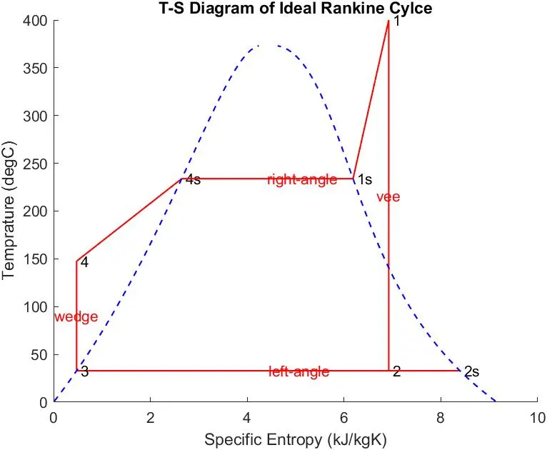
figure(1) % T-S
hold on
plot([S1 S2], [T1 T2], 'r', 'linewidth', 1)
text(S1,T1,' 1')
text(S2,T2,' 2')
plot([S2 S2g], [T2 T2s], 'r', 'linewidth', 1)
text(S2g,T2s,' 2s')
plot([S2g S3], [T2s T3], 'r', 'linewidth', 1)
text(S3,T3,' 3')
plot([S3 S4], [T3 T4], 'r', 'linewidth', 1)
text(S4,T4,' 4')
plot([S4 S1f], [T4 T1s], 'r', 'linewidth', 1)
text(S1f,T1s,' 4s')
plot([S1f S1g], [T1s T1s], 'r', 'linewidth', 1)
text(S1g,T1s,' 1s')
plot([S1g S1], [T1s T1], 'r', 'linewidth', 1)
plot(S_L, temp, 'b', 'linestyle','--','linewidth', 1)
plot(S_V, temp, 'b', 'linestyle','--','linewidth', 1)
%marking direction
text(S1,(T1+T2)/2,'vee','HorizontalAlignment','center','color','r')
text((S2g+S2f)/2,T3,'left-angle','color','r')
text(S3,(T3+T4)/2,'wedge','HorizontalAlignment','center','color','r')
text((S1f+S1g)/2,T1s,'right-angle','color','r')
title('T-S Diagram of Ideal Rankine Cylce')
ylabel('Temprature (degC)')
xlabel('Specific Entropy (kJ/kgK)')
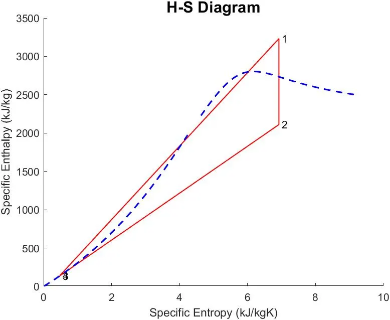
figure(2)
% H-S
hold on
plot([S1 S2], [H1 H2], 'r', 'linewidth', 1);
text(S1,H1,' 1')
plot([S2 S3], [H2 H3], 'r', 'linewidth', 1);
text(S2,H2,' 2')
plot([S3 S4], [H3 H4], 'r', 'linewidth', 1);
text(S3,H3,' 3')
plot([S4 S1], [H4 H1], 'r', 'linewidth', 1);
text(S4,H4,' 4')
plot(S_L, H_L, 'b','linestyle','--', 'linewidth', 1.5)
plot(S_V, H_V, 'b','linestyle','--', 'linewidth', 1.5)
title('H-S Diagram', 'FontSize', 15)
ylabel('Specific Enthalpy (kJ/kg)')
xlabel('Specific Entropy (kJ/kgK)')
Result:-
SIMULATOR OF RANKINE CYCLE
1-2 Isentropic Expansion in the Turbine
2-3 Constant Pressure Heat Rejection by the Condenser
3-2 Isentropic Compression in the Pump
4-1 Constant Pressure Heat Addition by the Boiler
Enter the Pressure at the Turbine Inlet (in bar): 30
Enter the Temperature at the Turbine inlet (in Degree celsius): 400
Enter the Pressure at the Condenser (in bar): 0.05
RESULTS
At state point 1:
P1 is : 30.000000 Bar
T1 is : 400.000000 Deg celsius
H1 is : 3231.571027 kJ/kg
S1 is : 6.923259 kJ/kgK
At state point 2:
P2 is : 0.050000 Bar
S2 is : 6.923259 kJ/kgK
X2 is :0.814256
T2 is : 32.875490 Deg celsius
H2 is : 2110.708212 kJ/kg
At state point 3:
P3 is : 0.050000 Bar
T3 is : 32.875490 Deg celsius
H3 is : 137.765119 kJ/kg
S3 is : 0.476254 kJ/kgK
At state point 4:
P4 is : 30.000000 Bar
S4 is : 0.476254 kJ/kgK
H4 is : 140.776056 kJ/kg
T4 is : 147.599058 Deg celsius
Work by turbine is : 1120.862815 kJ/kg
Work by compressor is : 3.010937 kJ/kg
Net Wok done is : 1117.851878 kJ/kg
Thermal efficiency is : 36.167131%
S.S.C is : 3.211811 kg/kWh.
Graph:-